Lesson 14 Waves and Maxwell’s Fields
Electromagnetic Waves
14.1 Contents
- A Little Bit of Maxwell
- Wave Goodbye
- Maxwell’s Idea of the Field: Maxwell’s Equations
- The Jelly of the Ether
- The Speed of Light, Old School
- Maxwell’s Insight and Electromagnetic Waves
- A Modern Summary of Maxwell’s Results
- So What Gets an EM Wave Going?
- The Lorentz Force, Broken Down
- Charged Particles in Electromagnetic Waves
- What to Remember from Lesson 14
14.2 Goals of this lesson:
- I’d like you to Understand:
How to predict the motion of a charged particle in a uniform electric field
How to predict the motion of a charged particle in a magnetic field
In words, not mathematically, what electromagnetic radiation is
- I’d like you to Appreciate:
The effort to put electricity and magnetism into a single, unifying theory
How accelerator magnets work
- I’d like you to become Familiar With:
The role of James Clerk Maxwell in the history of physics
14.3 A Little Bit of Maxwell
Dafty. That was his nickname as a kid at the Edinburgh Academy when he entered at the age of 10.
By the age of 14 he published his first mathematical paper on a generalization of an ellipse to include “ovals.” His consruction involved both a mathematical analysis and a physical model to draw the curves. This connection of the abstract and the concrete would reappear throughout hsi career. It was the first of three papers that he presented to the Royal Academy of Scottland…none of which were accepted for publication since the editors would not believe that someone so young could have actually done that work. He’d also published poetry before going to the university when he was 16 years old. Not ordinary.
After finishing his degree at the University of Edinburgh, he studied at Trinity College, Cambridge (Newton’s former home-base), graduating in 1854 at the age of 23. By the time he was 25 years old he held the chair of Natural Philosophy (“physics” in those days) at Marischal College in Aberdeen. That’s when he fixed Saturn and married Katherine Mary Dewar, daughter of the head of the college. They were childless, but their marriage was described later as, “married life…of unexampled devotion.”
A major prize was announced to explain why Saturn’s rings were stable. If they were solid, they should have broken apart. It took him two years to show that stability could only be achieved if the rings consisted of millions of small solid particles. They would all move together and clump in the way visible from a telescope…and only truly confirmed by the Voyager spacecraft in its Saturn fly-by in 1980. It’s now believed that the debris is left over from some moon of the planet that was broken up either through collision or enormous tidal forces. Said an examiner at the time of Maxwell’s submission, “It is one of the most remarkable applications of mathematics to physics that I have ever seen.”
Calculate it:Oh. He also did experiments to show that white light would result from the mixture of red, green, and blue light (aka “RGB”)—the principle that you’re likely experiencing on whatever computer display (CRT, LCD, OLED) you’re using to read this document.
SHY GUY
“At school he was at first regarded as shy and rather dull. he made no friendships and spent his occasional holidays in reading old ballads, drawing curious diagrams and making rude mechanical models. This absorption in such pursuits, totally unintelligible to his schoolfellows, who were then totally ignorant of mathematics, procured him a not very complimentary nickname. About the middle of his school career however he surprised his companions by suddenly becoming one of the most brilliant among them, gaining prizes and sometimes the highest prizes for scholarship, mathematics, and English verse.” as remembered by James Tait, a classmate and friend…and a pioneer of mathematical physics.
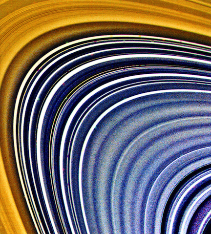
Figure 14.2: A Voyager 2 spacecraft saturn fly-by image of some of the rings. Voyager 1 is now leaving the solar system, traveling at a speed of \(3 imes\) the sun-earth distance per year.
He and Katherine moved to London in 1860 where he assumed the chair of Natural Philosophy at King’s College. During the six years he was there he did his most important work on electromagnetic theory, the subject of this lesson. He had read Faraday’s notebooks around 1855 and corresponded with the grand old man. But nobody anticipated what he’d do with Faraday’s ideas. While he was in London, he finally met Faraday. It’s quite pleasing to think about the 30 year old Maxwell and the 70 year old Faraday enjoying one another’s companionship and mutual respect.
In 1862 he wrote, “We can scarcely avoid the conclusion that light consists in the transverse undulations of the same medium which is the cause of electric and magnetic phenomena.” And in 1873 he wrote up his research in this area which was the enunciation of the four, fundamental Maxwell’s Equations that put everything together and form the basis of modern physics and relativity theory. It is a high-altitude summary of this work that interests us in this lesson.
Not content with his revolutionizing light and electromagnetism, he laid the foundations for the statistical basis of modern thermodynamics—what we call Maxwell-Boltzman theory today. He reluctantly found himself in the Chair at Cambridge University where he was the first Cavendish Professor of Physics in 1871. He designed the Cavendish Laboratory—in which we’ll see as the home of many 20th century milestones in the 20th century.
Unconscionably he became deadly ill with an abdominal cancer and died at the age of 48 in 1879. James Clerk Maxwell is always regarded as among the class of Newton and Einstein. Einstein wrote of Maxwell:
“[his work was the] most profound and the most fruitful that physics has experienced since the time of Newton.”
That he was as funny and companionable, as well as considerate as a supervisor rounds out a picture of one of the Big Three as being the most normal and highest quality individual among them. In these ways, he was perfectly matched for collaboration with Faraday, about whom nobody would say unpleasant things either—except about his presumed atrocious ideas. James Maxwell was indeed, Michael Faraday’s hero.
Let’s oscillate
14.4 Wave Goodbye
While the idea of an electromagnetic wave will change as we move into the late 20th century, there are some basic notions of waves that we’ll need. First doesn’t it make sense that we can think that all substances in the macroscopic world are either particles – or collections of particles – or waves.
Let’s think in terms of basics: the obvious features that distinguish particles and waves. It’s useful to think of idealized examples: an ideal particle will be one that’s infinitesimally small while an idealized wave extends in infinite directions and is perfectly repeating.
So, what is the most characteristic feature of a particle? That’s easy: Particles have a place, a definite location in space – it’s here. And furthermore, when it’s here, it’s also not simultaneously there. But a wave is everywhere, all the time. You can’t get much more different than that. It sounds almost like a distinction that only Aristotle could make, even if true.
But there are also tenuous similarities. Particles carry kinetic energy and transmit it through collisions with other particles. So too a wave is a disturbance that transmits energy. The tremendous destruction of a tsunami is terrible evidence of how energy can be imparted by waves. But the difference here is that the actual constituents of the wave don’t themselves translate but they stay put. This figure shows a finite disturbance like in a guitar string.
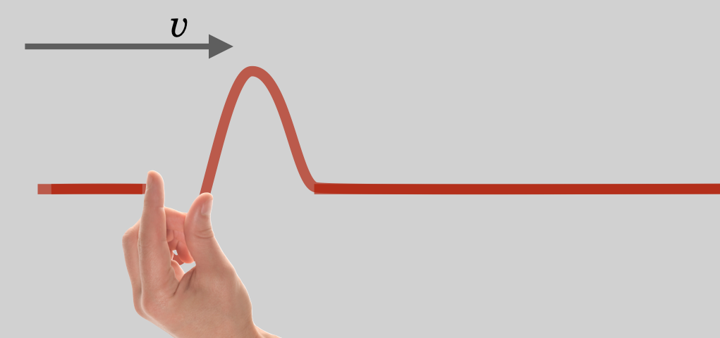
Figure 14.4: A “pluck” of a string transmits the potential energy of the displacement of the particles in the string through the tension and relaxation of the string. The disturbance moves away, while the bits of string stay put.
If you pluck a stretched string, you’ll create a disturbance that will actually move down the length of the string at a predictable speed where it would stop, or reflect and come back. If the string is attached to a bell clapper, it would ring. Obviously, energy and momentum have been transferred from your fingers through the string, sufficient to ring the bell.
Waves transmit energy.
It will be useful to think of waves as simple “sine waves.” That’s a simplification.(We will see later that any such non-repeating shape can actually be built up by a set of infinite sine waves of different wavelengths.) It’s also useful to contrast two kinds of waves: Longitudinal and Transverse.
- Longitudinal Wave: A wave in which the disturbance is along the direction of motion.
- Transverse Wave: A wave in which the disturbance is perpendicular to the direction of motion.
Longitudinal waves are compressional, like a slinky toy and appear in nature most readily in the propagation of sound. When a noise is made, the noisemaker vibrates and leaves a momentary compression or rarefaction in the surrounding air – a local high or low density region. This back and forth of high and low densities moves outward as the propagating sound wavefront. Actual molecules of the air don’t follow the wave all the way to your ear – local air molecules move and affect adjacent air molecules and that hand-off-disturbance is what propagates.
You eventually hear the sound, because that disturbance eventually reaches your ears and bangs on your eardrum like…a drum. Here is a cartoon showing two positions of a compressional disturbance along a spring-like substance.
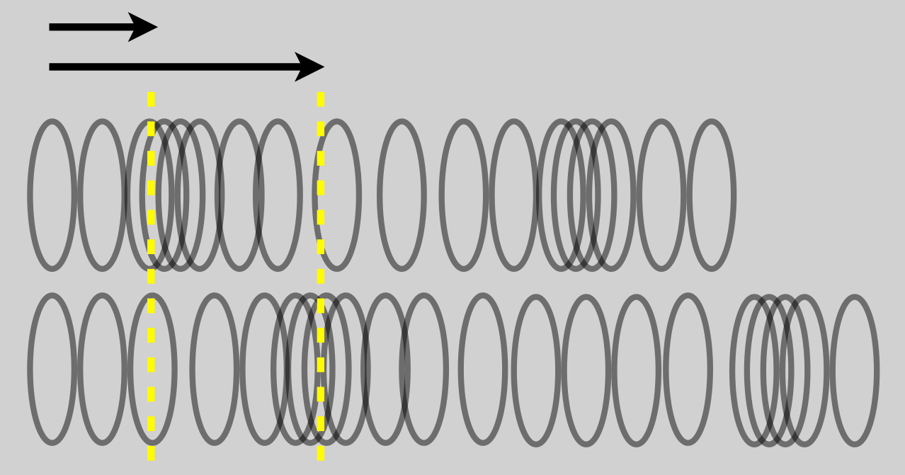
Figure 14.5: This is a longitudinal wave with the disturbance moving along the direction of the “slinky” and in the same direction as the speed of the wave.
Transverse waves are different in that the disturbance is not in the direction of the propagation, but perpendicular to it (that’s the definition of “transverse”). Water waves are the simplest example. If you toss a stone into a lake, the disturbance is the water going up and down but the wave propagates “outward” from the source in concentric circles. Again, the actual molecules of the water don’t move outward with the wave, the water molecules move up and down and affect adjacent water molecules through the tension in the water’s surface – rubber ducky just bobs up and down, he doesn’t follow the wave. This is a typical, infinite transverse wave. This figure shows a typical (infinite) transverse wave.
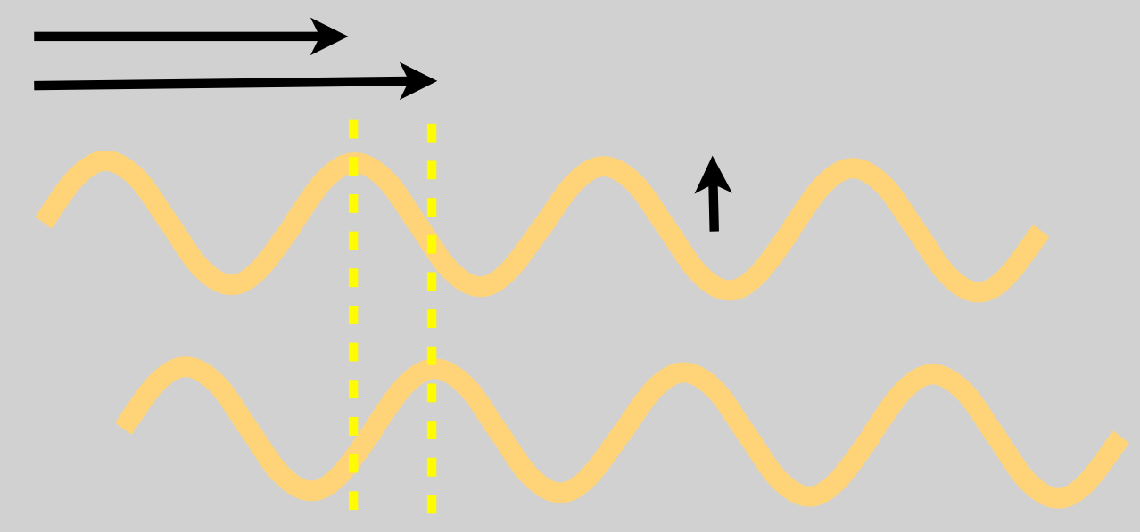
Figure 14.6: This is an example of a transverse wave where the disturbance is up and down but the propagation of the wave is along the length perpendicular to the disturbance, hence “transverse.” Notice that each peak (and valley…and every point in between) has moved to the right between the top and bottom snapshots of the wave.
14.4.1 Wave Parameters
We can characterize a moving sine wave with only a few parameters, which are are familiar from everyday life: frequency, wavelength, and amplitude. Notice that a wave is oscillating in space – you see the water wave undulate where the peaks are all in a pattern outward from the disturbance. But also a water wave oscillates in time where each point on the surface of the water is rising or falling in rhythm with all of the other points on the surface. That means we could plot the wave as either a pattern in space or time and the functional description of a wave would contain \(x\) and \(t\) variables.
🖋 📓
The next two figures show these two circumstances with three important features of waves indicated on each.
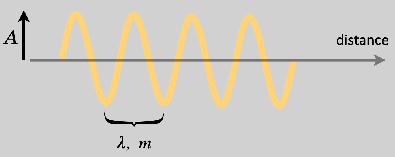
Figure 14.7: As a representation over distance, the disturbance varies with distance in a periodic way and the length of that repeating distance is the " wavelength," \(\lambda\).
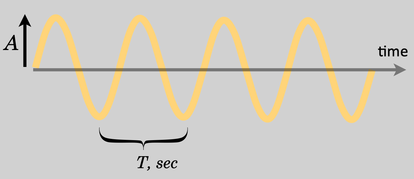
Figure 14.8: As a representation in time, the disturbance varies in time in a periodic way and the duration between points that repeat is the " period," \(T\).
The two most obvious parameters in the space picture are:
- wavelength, which is the distance in space units between any two equivalent values of the disturbance along the length of the wave (using the Greek letter, lambda \(\lambda\)) and
- amplitude, \(A\), the maximum disturbance which can be a length (like the height of water waves) or related to other measurable parameters like the value of pressure or light intensity or other not-so-obvious quantities like for electric and magnetic fields.
In the time picture there are also two obvious parameters:
- period, usually represented as \(T\)—which is the time that it takes for any same value of the amplitude to repeat (which is measured in seconds) and
- amplitude, the same amplitude as in the space picture!
The most common wave parameter – it’s on every radio dial – is the frequency which is the rate at which the wave repeats: the number of repetitions per unit time which has the units of \(s^{-1}\) or “per second.” This is given the name Hertz (Hz), after the great German physicist who first detected electromagnetic waves, Heinrich Hertz (1857-1894). House electrical current in the United States is a sinusoidal shape (alternating current, or “AC”) with a frequency of 60 Hz, or 60 cycles per second.
I’ll use the symbol \(f\) for frequency, although it’s also commonly represented as the Greek letter \(\nu\). (I don’t want to create any confusion with \(\nu\) for frequency and \(v\) for velocity.) Obviously, if the rate that the wave changes is \(f\) (“cycles per second”)and the time interval between the changes is \(T\) (“seconds per cycle”), then:
\[T=\frac{1}{f}\]
The space and time representations of the pictures of waves are connected by the actual speed of the wave (which makes sense since speed connects space and time!). This connection is the important relation (\(v\) is velocity!),
\[v = \lambda f.\]
Here are all of the parameters and their relations:
\[\begin{align} \text{Period of a wave: } \;\;\; & T=1/f \\ \text{ Speed of a wave: } \;\;\; & v=\lambda f \end{align} \]
With this introduction, let’s now see the light:
14.4.2 The Speed of a Wave
The speed of a wave depends on the medium, its density, temperature, structure, and so on. But, to first approximation, the wave speed doesn’t depend on the wavelength or the frequency (or the amplitude), so if the frequency goes up for some wave (like sound) because the speed stays the same, the wavelength goes down. High frequencies mean smaller wavelengths, and visa versa.
Electromagnetism is special. And this will be the rub for a really young Albert Einstein. The speed of electromagnetic waves in a vacuum is always (Here “always” will become a surprise.):
\[\begin{equation} v=3 \times 10^{8} \text{ m/s} = c.\end{equation}\]
The symbol \(c\) is reserved for that very special speed of light.
Wait. You’re always doing that: hinting at something to come.
Glad you asked. Yup. It’s a narrative trick, I guess. So many properties and features of nature were completely upended, that it’s fun to get you settled into something that’s comfortable and sensible and then rhetorically pull the rug out from under you later.
🖋 📓
Please study Example 1: Wavelengths for two familiar waves:
Our concern will be with the “electromagnetic spectrum” and here it is in its full glory:
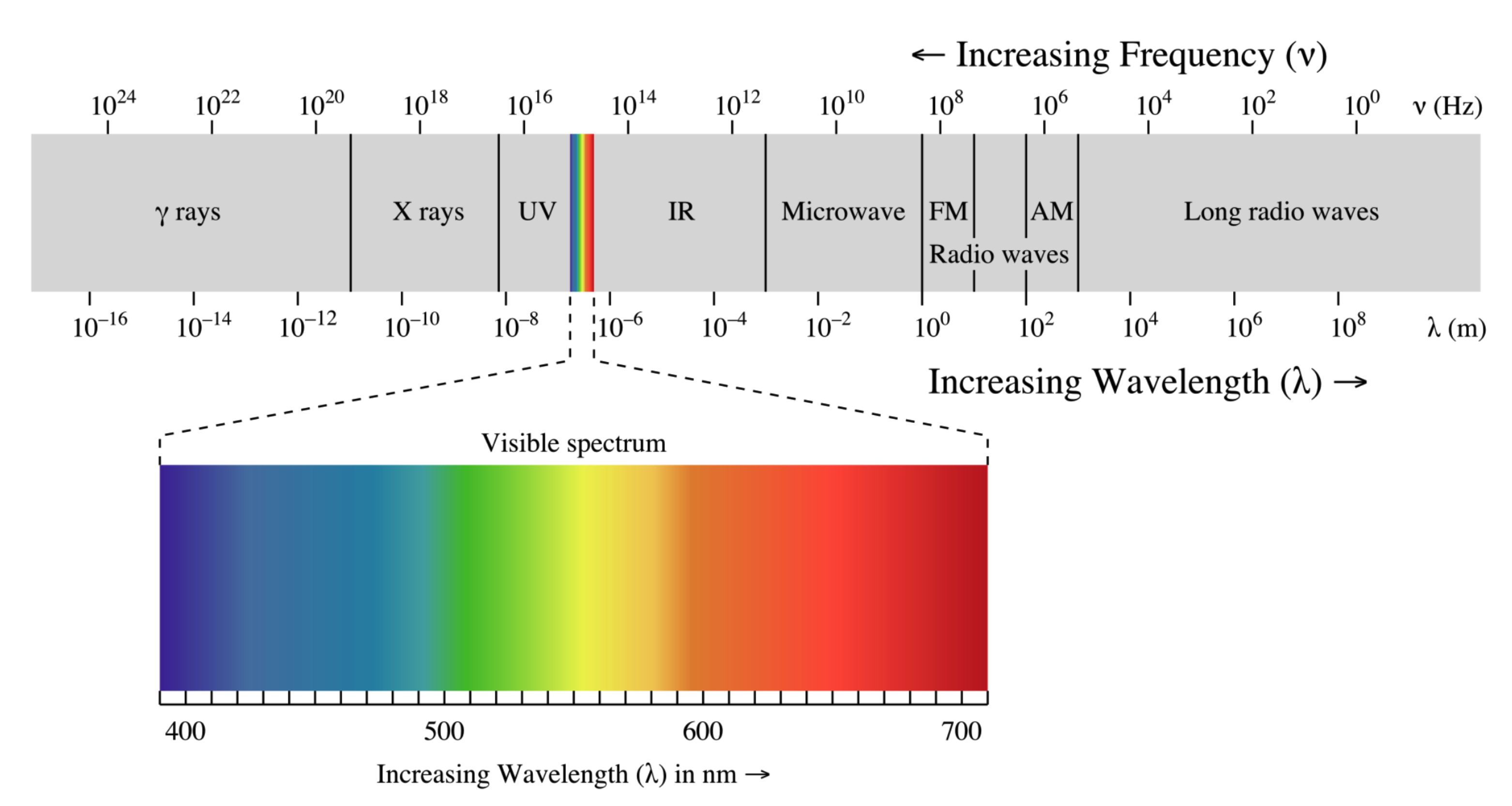
Figure 14.9: There are many phenomena that you have undoubtedly heard of and maybe didn’t realize we’re all the same thing. X rays, gamma rays, infrared rays, radio waves, and of course visible light waves…only differ by their frequency or by their wavelengths.
Electromagnetic waves all move at \(c\) so they can be characterized by either their frequency or their wavelengths. Notice that I wrote “rays” and “waves” which correspond to their everyday usage. This respects the history of their discovery as well see.
Wait. There you go again.
Glad you asked. \(\star\) crickets \(\star\)
14.5 Maxwell’s Idea of the Field: Maxwell’s Equations
The development of “Maxwell’s Equations” is a complicated subject and its historical roots are no longer relevant as you’ll maybe see. What Maxwell faced was the complete works of Faraday in electricity and magnetism which it’s worth summarizing, so that we face the same challenge as Maxwell.
14.5.1 The Four Electricity and Magnetism Challenges to Maxwell
Remember that Faraday studied quantitatively or outright discovered four phenomena:
- Electric charges create forces. Electrically charged objects (remember, at that time, macroscopically sized “chunks” of material) come in two forms arbitrarily designated as positive and negative.
- Attractive forces occur between oppositely electrically charged objects and repellant forces occur between same-charged objects.
- Faraday pictured the space between charges as consisting of material “lines of force,” actual material disturbances in space. He coined the term “fields” to this idea. This is the Electric Field.
- Prior to Faraday, Coulomb showed that the amount of force between two charged objects reduces by the square of the distance from them; separate them by twice as much, and the force will decrease by a factor of 4. This is the "inverse square" force relationship that gravity also respects.
- Magnetic poles create forces. Magnetized objects also come in two forms, historically dubbed as north and south.
- Forces are exerted between magnetic poles in a similar sense as for electrical charges; attraction for N-S poles and repulsion for N-N or S-S poles.
Unlike electrical charges, magnetic poles appear to always exist in pairs. Bar magnets cannot be separated into isolated magnetic charges (a phenomenon still with us today).
Although we didn’t consider this, Coulomb also showed an inverse square force relationship for magnetic poles.
Faraday came to his lines of force picture originally from his observation of the patterns of iron filings when in the presence of a magnet. It’s hard to not believe that “something is there.” This is Faraday’s Magnetic Field.
- Changing magnetic fields create currents. Faraday’s discovery of induction: a magnetic field that changes
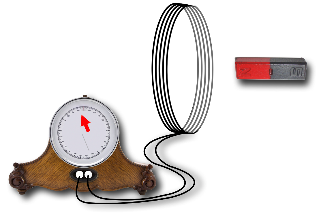
Figure 14.12: Reminder of the current induced in a wire ring from a moving magnetic field.
intensity in time will create a current in a nearby wire. When the magnetic intensity is constant, the current stops. This too could be restated as: “Changing magnetic fields create changing electric fields.”
- Currents create magnetic fields. Oersted’s discovery: electrical currents create a magnetic field (Faraday’s interpretation) that can exert a force on magnetic poles.
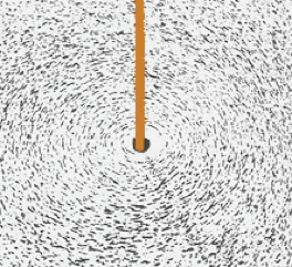
Figure 14.13: The circular magnetic field around a current.
Stay tuned to this last one.
The connection between electricity and magnetism was too intimate to be unrelated. Ampere and others had created mathematical models that ignored the field aspect, which was roundly dismissed by almost all of the community of physicists. For example, Ampere could calculate the force on a current-carrying wire by another current-carrying wire without reference to any field—just “action at a distance,” which was still as unsatisfying to 19th century people as in Newton’s time.
While Maxwell was still a student another genius student, himself only a few years older, William Thomson (the future 1st Baron Kelvin, OM, GCVO, PC, PRS, FRSE…whew) had worked out the mathematics of continuous heat and fluid flow.
Wait. Buried in that long list of titles, the Kelvin name sounds familiar
Glad you asked. Lord Kelvin, was one of the greats of late classical physics and one of only three people to have their own temperature scale named for them. There was Daniel Gabriel Fahrenheit, Anders Celsius, and Baron Lord Kelvin. The Kelvin scale has the same incremental size as Celsius (or centigrade) but its zero is at the absolute zero of temperature. You’ll find light bulbs’ color gauged on packages in “K”…5000K would be a bulb that has the color of bright daylight.
Thomson suggested, and Maxwell wrestled to the ground, the analogy that the equations that described the continuous flow of heat were similar to those that might describe the “flow” of electrical and magnetic fields…now proposed by Maxwell to be a continuous “flux” that the rate and direction of the direction of heat flow is analogous to the strength and direction of the “flow” of electric field. Just like heat can have a source (something hot) and a sink (something cold), the sources and sinks of electricity could be thought of as opposite electrical charges. You can sort of see this, right?
He took Faraday’s field idea and make it the actual “substance” of electricity and magnetism. He could account for both #1 and #2 above–static electric and magnetic fields with this direct analogy with heat or fluids. The time changing magnet and currents arrangements of #3 and #4 eluded him. But he thought he was onto something. He published his work in 1855, On Faraday’s Lines of Force.
In some ways, he’d not expanded on Faraday’s original “thought-pictures” but he did give them a respectable mathematical basis. Mind you: he was only a student, on his way to Cambridge! He was surely thrilled by the note he received from Faraday:
I received your paper, and thank you very much for it. I do not venture to thank you for what you have said about ‘Lines of Force’, because I know you have done it for the interests of philosophical truth; but you must suppose it is work grateful to me, and gives me much encouragement to think on. I was at first almost frightened when I saw such mathematical force made to bear upon the subject, and then wondered to see that the subject stood it so well.
The subsequent six years saw him complete his degree; receive (and lose) his job at Marishal College;22
become appointed as the Professor of Natural Philosophy at King’s College, London; receive the Rumford Medal of the Royal Society (for his color vision work); and election to the Royal Society (for color and for his Saturn rings work). It was time then to take up electricity and magnetism again, with an eye on those pesky #3 and #4 Faraday discoveries.
14.6 The Jelly of the Ether
Maxwell, along with virtually every natural scientist of the time, believed that light propagated as an undulation–a waving–of a substance that was everywhere: the “ether,” or more specifically for light, the “Luminiferous Ether.” It makes sense in a world where visible things are mechanical and if light is a wave, then something had better be waving.
So he made a model. Which evolved and which he then abandoned like a scaffolding that might hold up a new building until it’s no longer required and the building can stand on its own. It’s archaic, and frankly a little weird and so I’ll only sketch the idea.
Maxwell’s approach:
“I propose now to examine magnetic phenomena from a mechanical point of view, and to determine what tensions in, or motions of, a medium are capable of producing the mechanical phenomena observed.
”The author of this method of representation does not attempt to explain the origin of the observed forces by the effects due to these strains in the elastic solid, but makes use of the mathematical analogies of the two problems to assist the imagination in the study of both."
He was dealing with the odd notion that magnetic forces appeared perpendicular to the source of the force itself. That’s a little strange, right? If you push north on that red VW, you don’t expect it to move to the east. But that’s how things seemed to happen for magnetic forces. Remember Faraday’s moving magnet and the coil: move the magnet through the coil and the currents flow perpendicular to the magnet’s field, around the coil. Align two wires with currents flowing in them and the force that is produced is perpendicular to both the direction of the currents and to the direction of the magnetic field that one of the wires produces in the location of the other wire.
What, he thought, works that way in a mechanical environment? Spinning things. The axis of rotation of the earth is through the poles, but the bulge at the equator due to the centripetal force at that farthest distance from the axis is less and so the earth bulges at the equator–perpendicular to the spin axis.
So he built a model in which the magnetic field was due to little spheres of rotating masses. That they be massive was required because he needed them to bulge. (He presumed that the masses were so small as to not be apparent in real life–it’s a toy model, after all.) If the little spheres are everywhere, then the bulging of neighbors would create a pressure that’s perpendicular to their spinning axis.
But that creates a problem–ah, and an opportunity. Won’t the spinning of one row of spheres rub against the spinning of an adjacent row? Well it would, but what mechanical engineers do when there are adjacent spinning gears–and what Aristotle did with his crystalline spheres that supported the planets–is to add a row of “idler gears” which themselves rotate and translated that motion to the other row.
Here’s a set of drive gears and their shared “idler gear.”
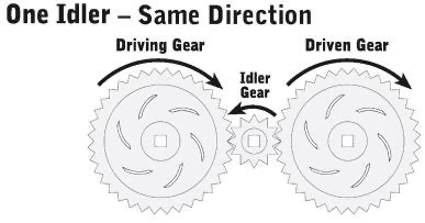
Figure 14.14: Idler gears transmitting the same rotational motion from one big gear to another.
Maxwell’s were not gears, per se, but spheres with adjacent friction to transmit motion. And what are they? Electrical charges in currents.
Here’s a picture from Maxwell’s eventual publication, On Physical Lines of Force The Theory of Molecular Vortices applied to Electric Currents in 1861 (part two of a four part series of papers, 1861-1862).
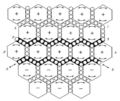
Figure 14.15: Maxwell’s odd mechanical model of fields and currents.
The two lines AB and PQ are physical, metal wires which consist of electrical charges that are free to flow. He imagines a voltage is applied between A and B and that these little spheres in the wires start to move. But, they’re idler spheres and so the cause the “molecules” in space or a material to begin to rotate on either side of AB. That’s the magnetic field surrounding a current-carrying wire and his picture is a slice through the spheres with their rotational axes pointing out or in.
Faraday’s induction: But there’s another wire just sitting there minding it’s own business between P and Q. That adjacent, now rotating set of molecules above AB are rotating and they cause the charges in the wire PQ to begin to move from Q to P. That’s an induced current–the current in AB caused a field which caused a current in PQ and he’s explained Induction. (Since a current creates a magnetic field, it’s a stand-in for the bar magnet in our oft-used example of creating a current in a loop in its presence.)
Furthermore, the rotating molecules are springy and that springiness he was able to imagine playing the role of the attraction and repulsion of electric and magnetic fields from static sources–attributing to space the ability to store energy (the elasticity of the springiness). So his model covers Faraday discoveries 1-3.
There’s a lot of work done by this little mechanical model of space.
In the course of four papers between 1861 and 1865 eventually the mechanical model went away, and the mathematical description remained. To this day, with one more additional suggestion that made all the difference.
But his model also predicted something that nobody’d considered before.
First, an interlude.
14.7 The Speed of Light, Old School
Let me remind you of two things. First there is the plain, ole’ electrostatic charge, say, positive.
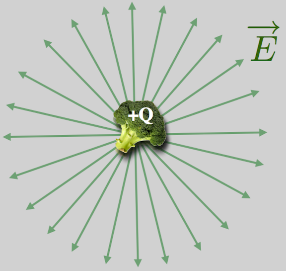
Figure 14.16: Reminder of the E field from a positively charged object.
Remember in Section 11 of Lesson 11 I remarked how both electrical and magnetic forces bore striking resemblences to one another and to the gravitational force. I described them generally as: \[ F_{12}=\text{Constant}\frac{\text{Source}_1\text{Source}_2}{R_{12}} \] For electrical forces, this looks like: \[ F_{12}=k_E\frac{\text{Q}_1\text{Q}_2}{R_{12}} \] and for magnetic forces it looks like: \[ F_{12}=k_M\frac{\text{m}_1\text{m}_2}{R_{12}} \] (Remember, that using \(m\) for a magnetic pole is hopelessly confusing with the use of \(m\) for mass in the gravitational force equation. Fortunately, I think I can count on one hand the number of times in my life where I’ve had to actually write something involving a magnetic pole! We won’t either.) The magnetic force was most prominently observed in the force between two current-carrying wires as described by Ampere. There, that same \(k_M\) occurs.
Both \(k_M\) and \(k_E\) could be measured! And they were by Wilhelm Weber and Rudolf Kohlrausch in 1855 in response to a paper that Weber wrote a decade before in which he described the combined forces between charges in a wire (the “electrodynamic” force) and a charge of an isolated electric charge (the electrostatic force). These combined forces–one electrical and the other magnetic were thought of correctly as both originating from electric sources, since a current is just electric charges in motion. Their measurement was a tour de force and Maxwell was aware of it. Weber and Kohlrausch even were able to determine that the ratio \[ \begin{align} \frac{k_E}{k_m} &= \frac{9 \times 10^9 \text{ Nm}^2/\text{C}^2}{1 \times 10^{-7} \text{ N}\text{C}^{-2}\text{s}^2} \tag{14.1} \\ &= 9\times 10^{16} \;\;\text{m}^2/\text{s}^2 \end{align} \] looked like the square of a speed, but of what Weber was unable to pinpoint physically because he lacked the insight that Maxwell provided. (Weber also had a \(\sqrt{2}\) misinterpretation.)
Armand Hippolyte Louis Fizeau, a Frenchman with a very impressive name, did an incredibly impressive experiment in 1849 which measured the speed of light to be \(3.133 \times 10^8\) m/s. Pretty close to the square root of \(k_E/k_M\) above.
By the way, it is from Weber’s original paper that we get the symbol “\(c\)” for the speed of light.
14.8 Maxwell’s Insight and Electromagnetic Waves
Let’s look at basically what bothered Maxwell. First, remember that a current, which means a changing electric field, is generated when a magnetic field changes in time. That’s the current loop above, where the electrons in the wire move because of the magnetic-field-induced electric field pushing them.
Let’s look at two metal plates that are connected to wires in a circuit. Maxwell thought of the region between the plates as consisting of actual non-conducting material (called a dielectric) and the whole device is a circuit element called a capacitor, about which we’ll have more to say below. For now let’s just be simple–by even more strangely imagining that there’s nothing between the plates.
Here’s the picture: a battery, a switch that’s closed, and our plates. Simple, but odd as we watch what happens as time passes.23
In the top figure, we close the switch and current begins to flow. Remember:
- the convention is that current flows from the positive terminal of a battery to the negative. The arrows signify that.
- in actuality, the actual current is electrons in the wire which are repelled by the negative terminal of the battery and go in the opposite direction of the conventional current. I’m just the messenger. Blame Ben F.
In the bottom figure, you can see that the flowing current creates a circular magnetic field around the wire with the direction indicated.
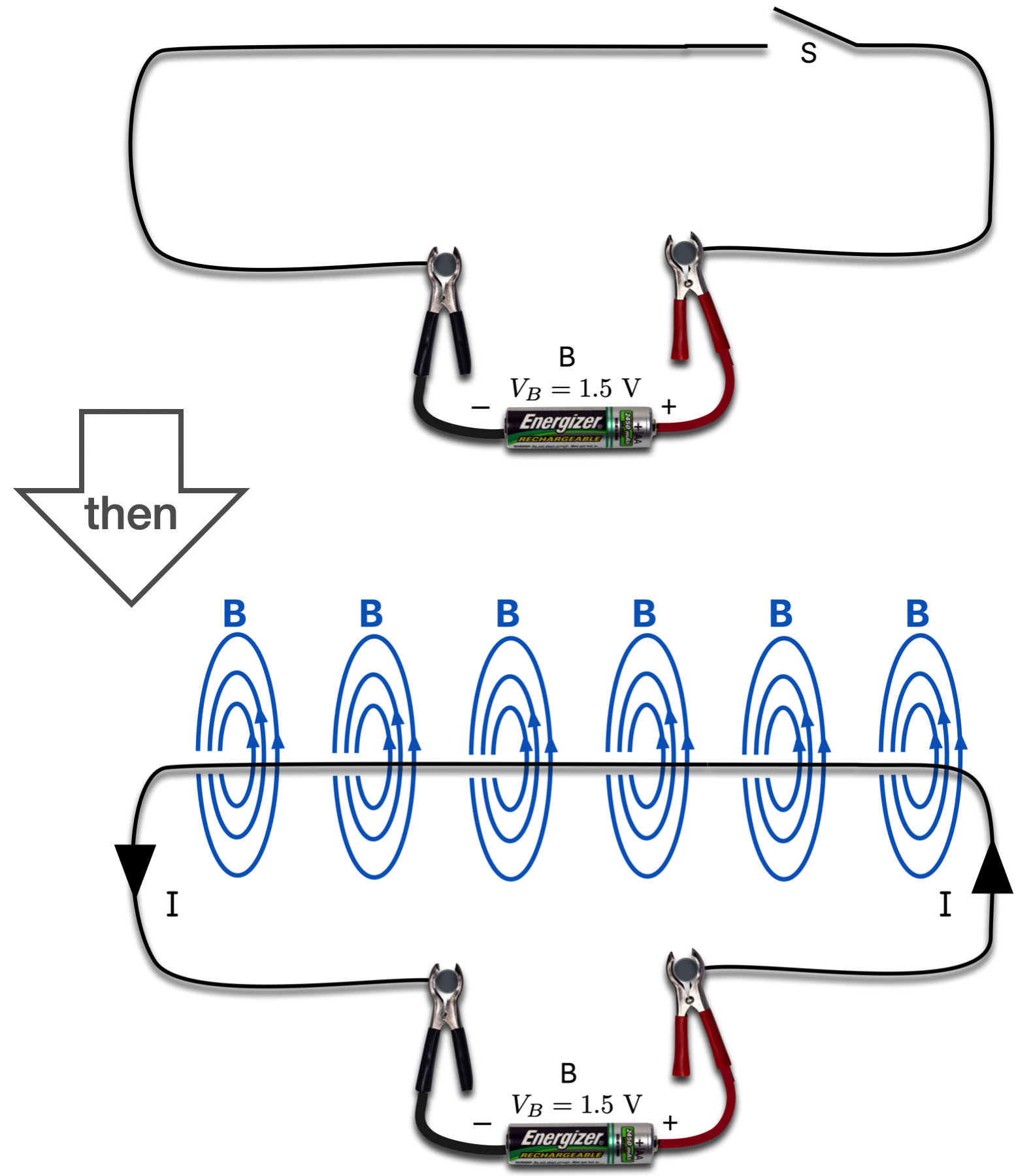
Figure 14.17: At the top, a switch is open and no current flows. At the bottom, the switch is closed and the current creates a magnetic field circulating around the wire throughout.
Now let’s add a circuit element to the picture, namely two metal plates and a gap between them…called a capacitor. We can collect charge on a capacitor by connecting it across a batter like shown. In the bottom figure, the switch has been closed and current starts to flow. But:
- There’s a gap! So charges don’t flow from P2 to P1 (unless it sparks, which is an unwanted current in most circuits!)
- So we see that the charges in the whole circuit start to arrange themselves so that electrons build up on P2 and leave P1…leaving an overall positive charge on P1.

Figure 14.18: Now a circuit is interrupted by two parallel, metal places and a switch. The plates are a circuit element called a ‘capacitor’ used to store charge. In the top the switch is open and nothing happens. Then the switch is closed and the bottom figure shows what starts to happen. As current flows, a magnetic field develops where current is flowing. That current is interrupted by the plates which begin to store charge on their surfaces.
On can picture the electrons building up on the right hand plate (Remember the current flows in the opposite direction of get actual conducting electrons. Thanks, Ben.) and how the left hand plate is robbed of electrons and becomes positive.
- This charge build-up happens over time.
Look at the situation below as time goes on. We start from no current and no voltage across P2-P1 (\(V_P\)). Then after the switch is closed, current starts to flow and that charge build-up happens…a little (lower left)…and then more…lower right. At each of these two stages, the voltage builds on the plates and the electric field between them gets stronger and stronger.
Notice how unsatisfying this magnetic field is: it just goes blank at the edges of the plates. It’s discontinuous and in some sense Maxwell found that his model would fix that!
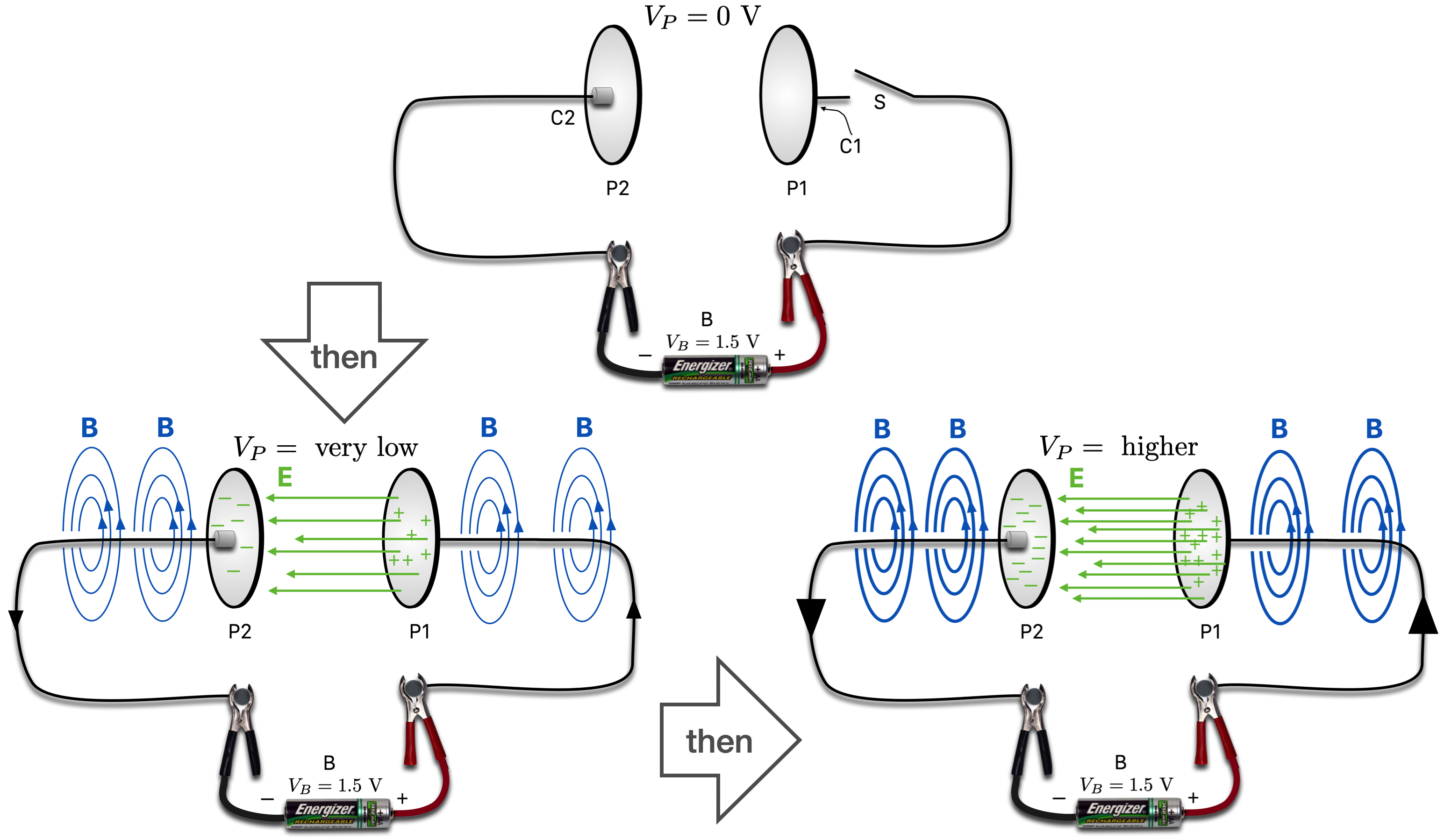
Figure 14.19: This is the same situation as in the previous figure, but in the bottom two sketches, the electric field is shown developing between the plates. As more current is delivered, the magnetic field gets stronger and the electric field (confined to between the plates) gets stronger. A voltage develops across the plates getting bigger as more charge is deposited.
Let’s continue to let the current flow and come back to that unpleasant gap of magnetic field.
The top figure below is just before the voltage across the gap matches that of the battery. When than happens, that balance means that there’s no incentive for the electrons to flow and:
- the current stops flowing
- \(V_P=V_B=1.5 \text{ V}\)
- and without a current, the magnetic field goes away and we’ve got a stable situation.
- But: there’s now a static electric field left between those two plates.
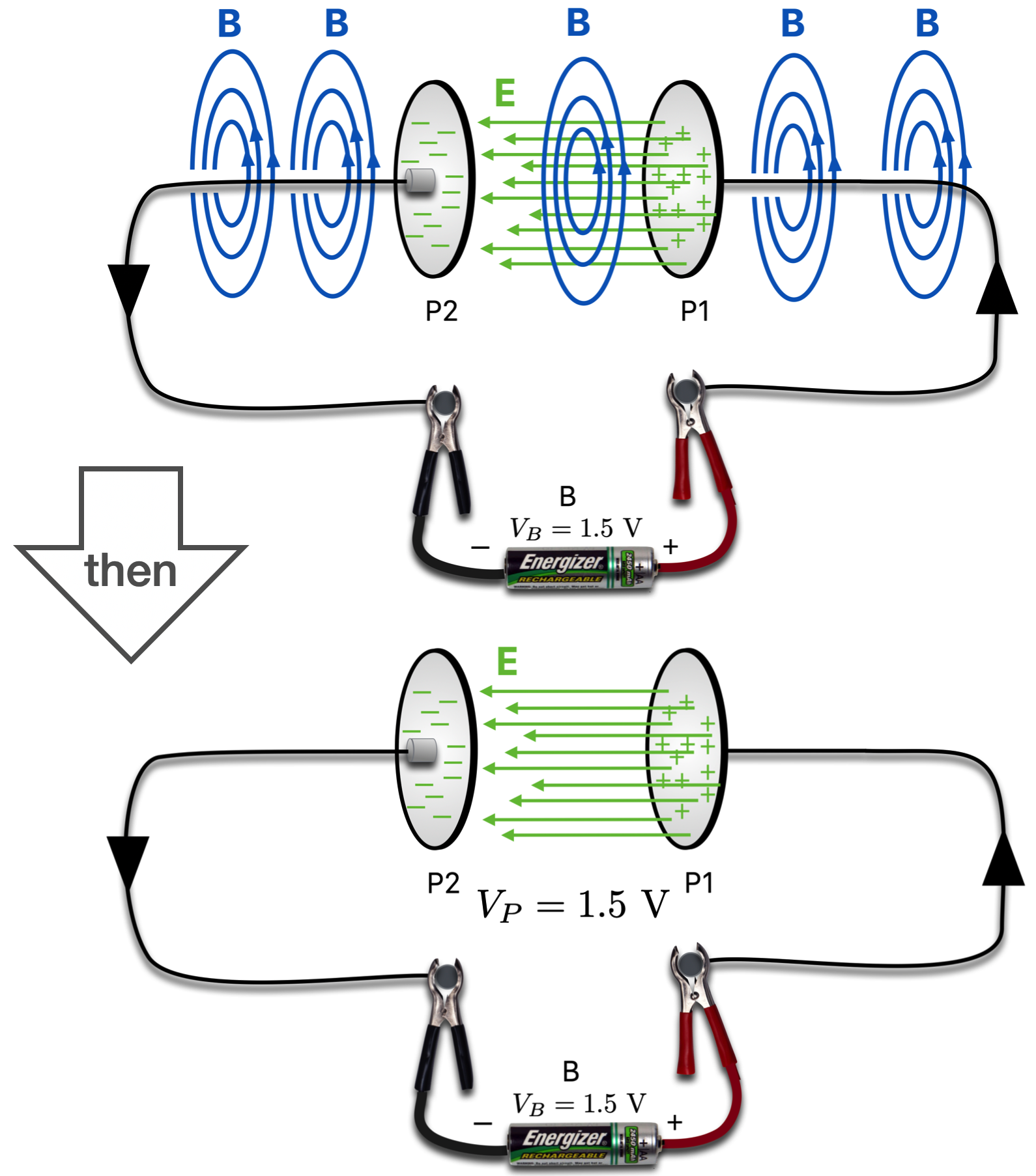
Figure 14.20: But the discontinuity of the magnetic field is bothersome and Maxwell’s model responded. There is a magnetic field between the plates also as suggested in the top. Eventually the charge deposited on the plates leads to a voltage across the plates that’s equal to the battery voltage. When that happens, the current stops flowing: the magnetic field disappears and the electric field remains.
Now about that strange discontinuity of the magnetic field. Look at Maxwell’s mechanical picture again:
Figure 14.21: Maxwell’s mechanical model again, showing little currents tha that are not flowing inside of wires: like P-q.
Notice that there are other idler spheres that are not connected to any external circuit in this model. They are not “real” currents and don’t actually transmit real electrical charges–but the act like little currents. Maxwell called them “displacement currents” and proposed that between those plates, they were in action:
- although no currents actually transmit charges, there is an effective–even “fictitious” current called the “displacement current,” \(i_d\).
- if you’ve got a current, then you’ve got a magnetic field! And so he preserves the continuity of the magnetic circular fields through the gap by pretending that there’s a strange, displacement current.
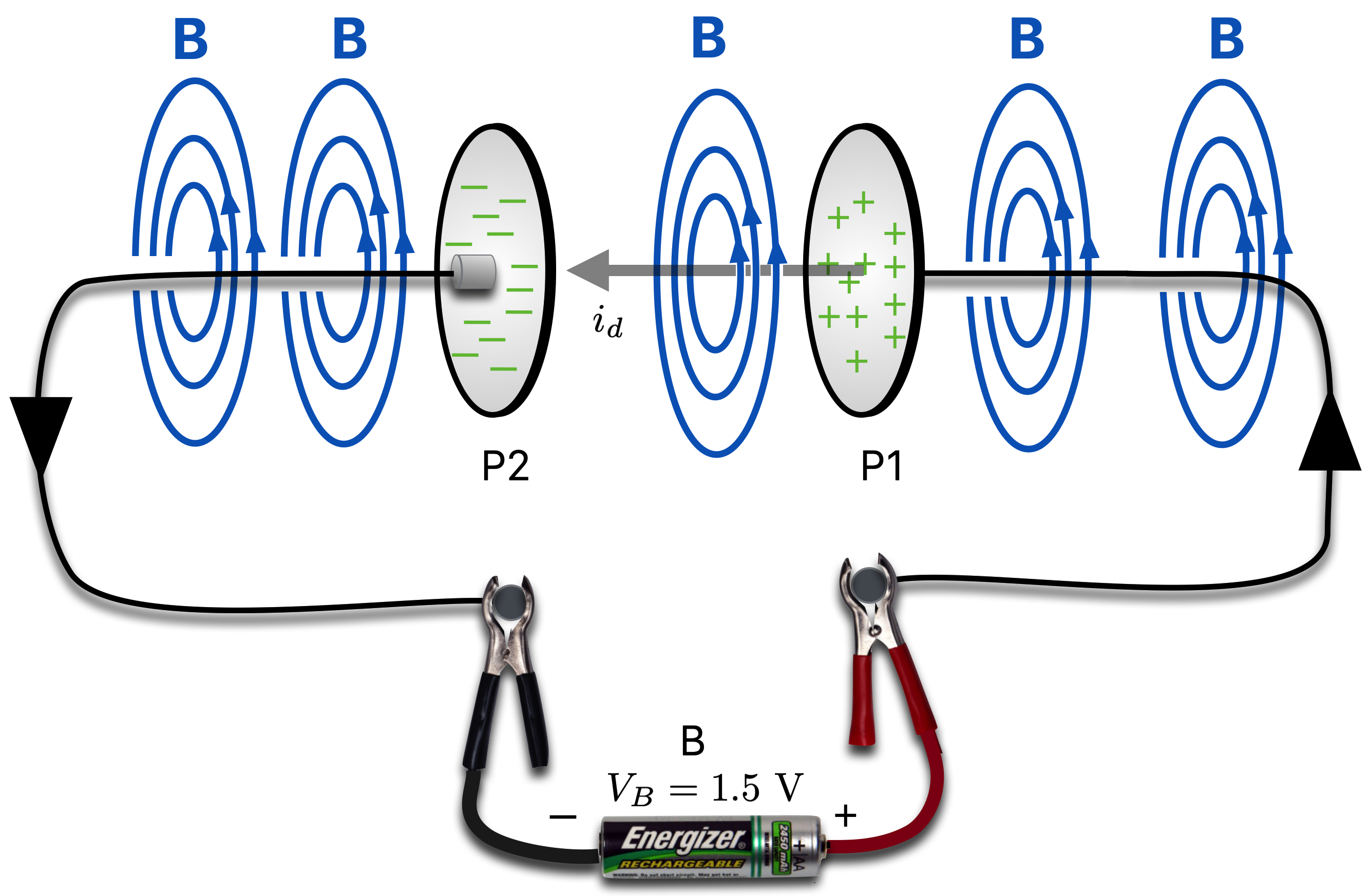
Figure 14.22: Maxwell posited the existence of the ‘displacement current’ that flows without actual charge exchange between the plate. As a ‘current’ it might generate that missing between-the-plates magentic field. But it’s more concreted to tie the existence of the magnetic field to the changing E field and not to the displacement current.
But what’s really going on is that there’s that changing electric field between the gap:
- That E changes as the current charges up the capacitor
- It’s responsible for the displacement current
- which is responsible for the (changing) B field
- But why not just get rid of the middleman, that displacement current?
It’s the changing E field that creates that inter-gap changing B field.
Now, he’s added to the picture: not only does a changing magnetic field create an changing electric field, but a changing electric field creates a changing magnetic field.
He had 20(!) equations, each of which described the four phenomena listed at the beginning of this discussion. But they were asymmetric originally with a changing magnetic field featuring prominently in #3. Now, there’s a corresponding changing electric field creating its partner magnetic field in #4.
This makes the sum total of that set of equations have solutions which were familiar to all physicists of his and our time. These solutions are waves. There is a solution that describes a time-waving electric field and another one that describes a time-waving magnetic field.
And. They are linked together. One of them creates the other…and the other creates the former:
A changing E field creates a changing B field
which in turn creates a changing E field
which in turn creates a changing B field
which in turn creates…and so on
This is an electromagnetic wave and the velocity at which that wave propagates is:
- perpendicular to the directions of the two perpendicular E and B vectors
- and has the magnitude of \(c = 3 \times 10^8\) m/s
This is what Weber missed. His speed had no physical interpretation. Maxwell provided the missing piece…and then he took away the “scaffolding” of the mechanical spinning balls and let the equations stand on their own.
Maxwell, in his 1864: A Dynamical Theory of the Electromagnetic Field
“The agreement of the results seems to show that light and magnetism are affections of the same substance, and that light is an electromagnetic disturbance propagated through the field according to electromagnetic laws.”
His 20 equations were made more succinct by Oliver Heaviside into four vector differential equations which all physicists and engineers revere as “Maxwell’s Equations.”
That Maxwell’s Equations predicted waves with a speed equal to the measured speed of light meant that light is composed of electricity and magnetism.
Maxwell’s equations unified optics, electricity, and magnetism into a single model of nature: Electromagnetism.
His death at the age of 48 in 1879 was tragic for his family and friends, but also a depressing conclusion to the Maxwell story. The distinct prediction of electromagnetic waves was to await confirmation until 1887, less than a decade later. After two years of work, the young, but brilliant Heinrich Hertz (for whom we name the frequency of wave motion), was able to detect the wavelike nature of radiation from sparks (which are visibly bright, but also “bright” in other wavelengths) and actually measure the wavelength of the light that traversed the length of his lab. Hertz himself was to die tragically at the age of 36.
What Hertz confirmed was that an electromagnetic wave is a coupled arrangement of mutually-inducing oscillations of magnetic and electric fields moving together at the speed of light. Here’s a cartoon:
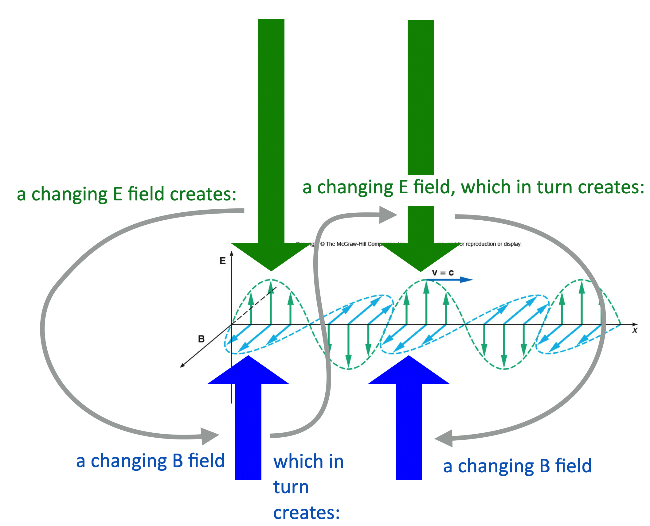
Figure 14.23: The mutual creation of electric and magnetic fields—one changes in time creates the other changing in time, which in turn, creates the first…and so on. All from the solutions to Maxwell’s Equations.
The electromagnetic wave is moving to the right. You can see the oscillating fields, E up and down and B in and out. The Changing E field creates a changing B field…and that changing B field in turn creates its partner changing E field…and so on and so on. Furthermore, their magnitudes are related: \[ \frac{E}{B}=c \nonumber \]
14.9 A Modern Summary of Maxwell’s Results
Maxwell not only unified three different fields into a single theory, but his prediction was that there were entirely new electromagnetic wave phenomena beyond just what we can visibly see with our eyes. In fact, “light” is only a tiny portion of what’s called the Electromagnetic Spectrum. Here it is in all of its glory:
Figure 14.24: The electromagnetic spectrum.
An electromagnetic wave (E&M wave) is a transverse wave with two coupled amplitudes of an electric and magnetic field vector traveling at a single speed, that of light: \(c=3 \times 10^8\)m/s. Your cell phone signal? E&M waves. The light through your window? E&M waves. The warmth you feel on (and radiate from) your skin. Yup, E&M waves. Back and forth. We’ll see that even the teenage Einstein found a contradiction here that in part stimulated his venture into Special Relativity.
You shield yourself from the sun’s rays because not only does the sun shine visibly, but it emits short-wavelength electromagnetic waves which we call “ultraviolet.” Something is hot–and you’re warm–because any object and you emit infrared radiation which we perceive of as heat. In fact everything in your life emits radiation of all different sorts and all of them are identical in one important way:
All electromagnetic waves travel at the speed of light.
Because any wave’s speed, frequency, and wavelength are all related by one simple relation: \[ c=f\lambda \tag{14.2} \] the only thing that distinguishes the color blue from infrared waves or radio waves or microwaves are their wavelengths, or equivalently, their frequencies–again, because they all move at the same speed.
Now that’s we’re friendly with Electromagnetism, we can call it by its nickname: EM.
14.10 So What Gets an EM Wave Going?
I’m glad you asked. Imagine a positive charge just sitting still in front of you minding its own business. Think about the field that results from that stationary (relative to you) charge: it’s just our now familiar E field pointing radially away.
Now let’s imagine that the charge is moving by you at a constant speed. What are the fields now? Well, you’d still see the E field, but now that moving charge is a current and so there’s be the familiar circular B field around it as it moves.
Now: apply a force to that charge so that it accelerates. Its changing speed–the definition of acceleration after all–causes a kind of kink in the fields. That kink propagates outwards and is in fact, an EM wave.
An accelerated electrical charge creates an Electromagnetic wave.
What’s a broadcast antenna? Well, it’s nothing more than a wire in which electrons flow, driven by a source of energy that causes those electrons to accelerate up and down. Those accelerating electrons produce EM waves that propagate outwards: that’s your favorite radio station.
Meanwhile somewhere in your car or your home, you’ve got another wire which is sitting there with its electrons idling their motors waiting to be tickled. When that EM wave from the radio broadcast antenna pass by, the electric fields in them apply forces to those electrons in your receiving antenna and the electronics in your radio transform those oscillations into Lady Gaga’s voice.
###Energy
It takes energy to apply the forces to the electrons in the broadcast antenna and energy is clearly applied to the electrons in your radio’s receiving antenna. So obviously, the EM wave that’s in-between carries energy from one place to another. Faraday anticipated this and Maxwell modeled it in his elastic “molecules” but today we know that EM waves contain and deliver energy.
🖥️
Please answer Question 1 for points: Changing E field:
🖥️
Please answer Question 2 for points: Changing B field:
🖥️
Please answer Question 3 for points: Stationary magnet/coil:
🖥️
Please answer Question 4 for points: Moving magnet into coil:
🖥️
Please answer Question 5 for points: Moving magnet…again:
🖥️
Please answer Question 6 for points: E and B?
14.11 Charged Particles in Electromagnetic Fields
It’s charged particles from here on…
Atomic particles were not a useful concept during the mid-1800s. Chemists were beginning to organize themselves around atoms and molecules, but few actually argued for the actual existence of unsee-able states of reality. So it wasn’t until the last decade of the 1800’s where the urge to think this way became acceptable–to some.
We will consider J. J. Thomson quite a bit later–he is credited with the discovery of the election (for which he won the Nobel Prize) and from an early age was predisposed toward the possibility that matter consisted of minute, identical charged entities–like the electron. He was also credited as being a brilliant scientific administrator and dangerous with laboratory equipment! His co-workers tried hard to keep him away from delicate instruments.
In 1881 he was the first to try to use Maxwell’s Equations to calculate the force on a charged particle due to a magnetic field. He got it wrong in the details, but essentially correct in the form. The socially awkward Oliver Heaviside, who took Maxwell’s 20 equations and created the vector calculus necessary in order to deal with only four, fixed Thomson’s mistake but it was the Dutch theoretical physicist, Hendrik Lorentz who put the whole thing on a formally correct basis: charged particles experience forces from both electric and magnetic fields and this combined force can be described in a simple model.
The force that an electric field causes on a particle with electrical charge \(q\) we’ve already encountered:
\[ F_E= qE \] Remember that the force direction is “signed” in this equation: if \(q\) refers to, say an electron where \(q=-e=-1.6\times 10^{-19}\) C, then we’d have \[ F_E= -eE \] and the negative sign would point would indicate that the force points in the opposite direction to the electric field vector direction.
What Thomson derived with a mistake and Lorentz and Heaviside fixed was the force on a charged particle due to a magnetic field. It’s \[ F_M=qvB \] where \(v\) is the speed of the particle of charge \(q\) and here the assumption is that the velocity direction is perpendicular to the B field direction…and the mathematics of vector calculus tell us that the force that \(q\) experiences is perpendicular to the both of them. Here your right hand tells you the direction.
That speed is waiting to cause trouble
The \(v\) in this relation is the speed of whatever charged particle is experiencing the forces. You might ask, “speed with respect to what?” and you’d be correct to do so. Remarkably only the very young Albert Einstein asked that question in his patented style of asking scientific questions and found that the answer turned Newton upside down. What Lorentz and everyone before Einstein said was that this speed is with respect to the Luminiferous Ether in which EM waves all traveled at the speed of light. Much more on this when we get to Relativity.
14.12 The Lorentz Force, Broken Down
Let’s go back to the forces between two wires carrying currents and let’s break it down to the actual particles involved in a current and the magnetic field that they produce.
Remember that we saw that two parallel wires carrying current in the same direction would feel a force of attraction and physically move. Now we’re going to understand why. Here we’re concentrating on the force that wire B feels due to current A, \(F_{BA}\).
This example will walk you through this:
🖋 📓
Please study Example 2: The Lorentz force explains the force between current-carrying wires
14.12.1 Charged Particles in the Presence of Electric and Magnetic Fields
When an electric charge is in the presence of an electric field, as we know it experiences a force along the direction of the E field lines if it’s a positive charge, and against the direction of the field lines if it’s a negative charge. So in this figure the positive charge goes up and the negative, down.
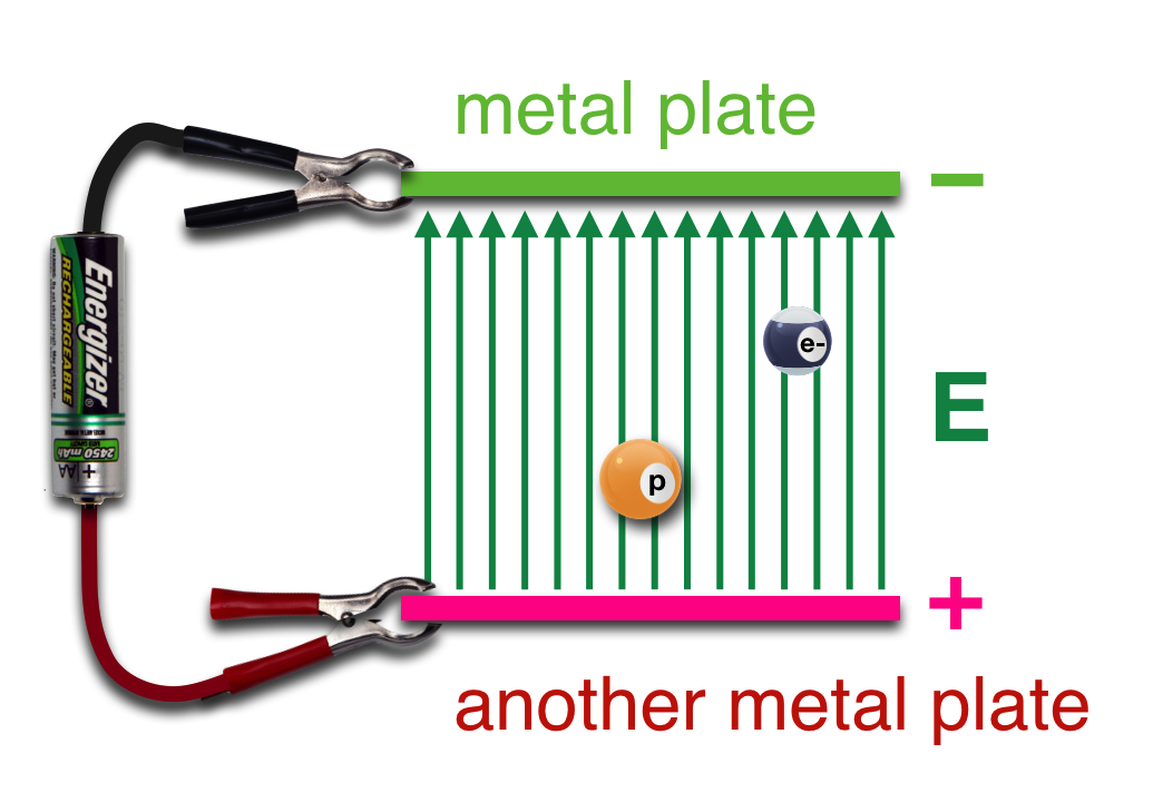
Figure 14.27: A cross section of two metal plates with a voltage across them. The electric field will apply the same magnitude force to a proton and an electron (because they have the same electrical charge magnitude) but in opposite directions: proton, up, with the field and electron, down, away from the field.
Magnetic fields are different. If you put an electric charge in a magnetic field…nothing happens. That stymied Faraday until he moved the magnetic field relative to the charges in a current loop–which is the same thing as moving an electric charge in the presence of a stationary magnetic field. Then, it feels a force.
Let’s build a magnetic field distribution without worrying how we do that (stay tuned). Here in (a) we have a magnetic field that’s pointing up and extending out at you and into the screen–it’s in three dimensions. We’re looking at it with the B field arrows pointing right at us. In (b) we’ve changed our vantage point so that the B field lines point into the screen right toward us. Get the picture?
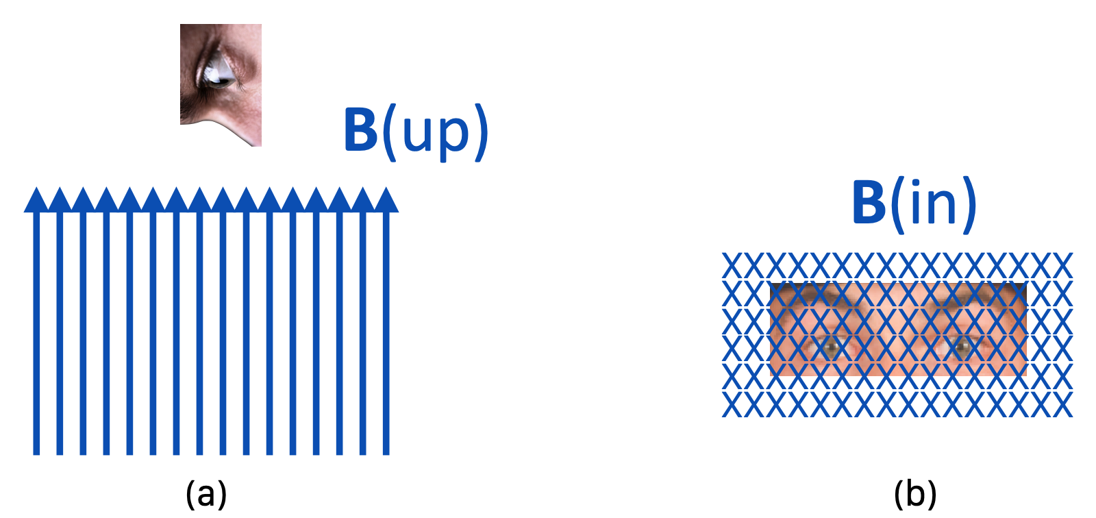
Figure 14.28: In the left, a magnetic field is pointing up, toward our gaze. In the right, the field is shown from behind, still aimed at our view.
Now let’s shoot a positively charged particle into that B-in oriented field so that its velocity is pointing to the right.
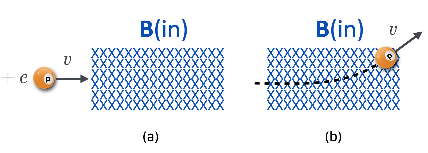
Figure 14.29: A positively charged particle comes into a region with a magnetic field from the left and when it encounters the field, it bends up, due to a force that’s perpendicular to both the proton’s velocity and the magnetic field direction.
It feels a force, but perpendicular to both the field and its velocity–it bends! In this case up. That’s what magnetic fields do to electric charges. It bends their trajectories–the charge has to be moving and then it’s susceptible to a bending force.
An electric charge which is moving relative to a magnetic field will experience a force which is perpendicular relative to its velocity and the direction of the magnetic field.
The value of the force is an important calculation if you build particle accelerators (or old-time TV sets). We’ll only need to know how to determine the direction of the bend.
The relevant quantities to determine this are the three vectors: \(\vec{v}\), \(\vec{B}\), and \(\vec{F_M}\) (the magnetic force) and the electric charge sign, \(+\) or \(-\). This is a job for vector algebra, for which we’ll need a hand. In particular your right hand and this is another application of a “right hand rule.”
There are a couple of ways to use your right hand to figure out the direction of a force and the order of \(\vec{v}\), \(\vec{B}\), and \(\vec{F}\) are important. Here’s probably the easiest one of…–dare I say a “handful” of right hand rules. Take your right hand and its index finger pointing out. Take your second figure and make it go perpendicular to your index finger (it only bends one way, unless you’re built strangely), and then extend your thumb in the only direction that it can go.
- Your index figure is the \(\vec{v}\).
- Your second finger is the \(\vec{B}\).
- Your thumb points in the direction of the resulting \(\vec{F}\).
Look again at the bending charge that we just sketched, now with some assistance. Notice that the B field direction is in, so the third finger is pointing into the screen.
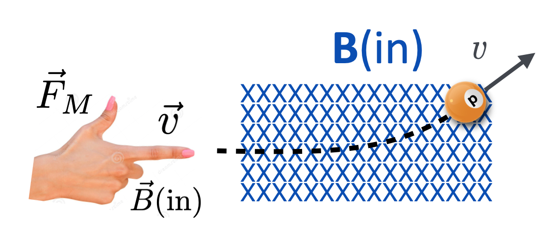
Figure 14.31: How we get the upward-bending force on that proton.
You might need to play with this a little. If you do it on the bus, people will stare, but try to look at both the perspective figure and the from-the-top figure and confirm that the force is where your thumb wants it to be.
So now we have what’s called the “Lorentz Force.” It’s the combination of the force on a charge experiencing an electric field and the force on a charge experiencing a magnetic field. \[ F=q\vec{E} + q\vec{v} \times \vec{B} \] That \(\times\) sign symbolizes the very special kind of multiplication of vectors called a “cross product.” For us, that’s just saying, “get out your right hand and do the thing with your three fingers!” In order: \(\vec{v}\) then \(\vec{B}\).
Suppose this had been an electron, so that the charge was opposite of that proton? Then the force would point in the other direction since the electrical sign will become a vector sign.
Wait. Then what about the current, doesn’t that mean that the wires will separate?
Glad you asked. Remember that if we think about the current as an actual wire-carrying-electrons situation not only does \(q\) become negative, but also the velocity changes direction so that the overall sign is the same as what we constructed. Good question, though.
Now we can build a particle accelerator. We start with protons or electrons (or nuclei) and inject them into a region of an E field. That accelerates them. They leave the accelerating region and enter a carefully crafted magnetic field region designed to bend the particles in the direction of an experiment.
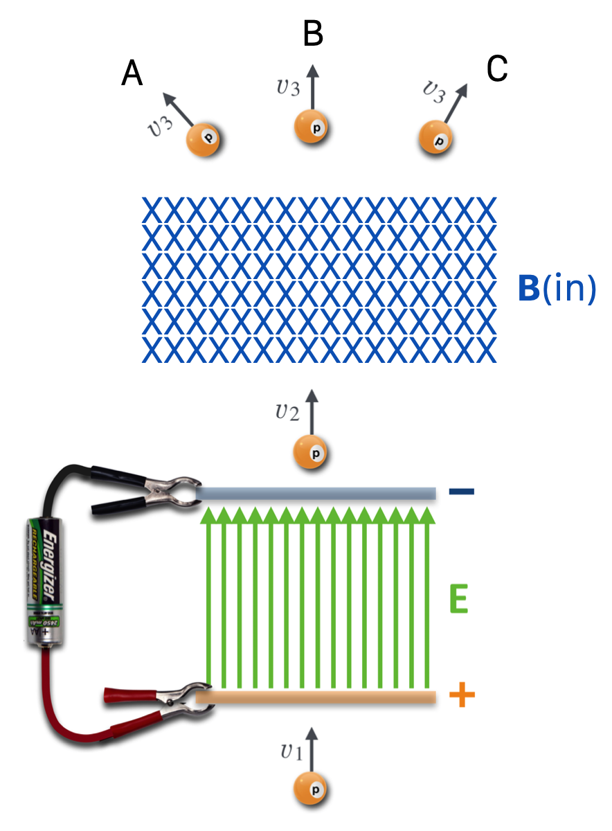
Figure 14.32: A litle particle accelerator: speed up a proton and then bend it to where you want it to go. Which direction? A, B, or C?
Can you see that the bending of that beam of protons would be to the left, A?
Now we understand the Aura Borealis, the “Northern Lights.”

Figure 14.33: The auroa borealis. The stranded colors of de-exciting atoms show the tenuous magnetic field lines of the upper atmosphere.
The Earth’s magnetic field is concentrated at the north and south poles. It’s necessary for our survival because our Sun can be an angry neighbor. The charged particles near the surface of the Sun have varying speeds and some small fraction of the protons and electrons at that surface actually are above the escape velocity and off into space they go–this is the “Solar Wind.” The Sun’s solar storms can send whole swarms of charged particles that our Earth’s path might intersect.
But those charged particles get trapped in the B field lines of the Earth and spiral (that’s the \(v \times B\) bending at work) toward the pole. As the field gets tighter near the pole the rotational speeds of the particles increase enough to excite the Nitrogen and Oxygen in the upper atmosphere which, when they de-excite emit light, green for Oxygen and blue and red for Nitrogen.
14.13 What to Remember from Lesson 14
14.13.1 Waves
The wavelength (\(\lambda\)), frequency (\(f\)), and speed (\(v\)) of a wave are all related through a simple model:
\[v=\lambda f.\]
14.13.2 Electromagnetism
James Clerk Maxwell found mathematically that
- a changing magnetic field would induce changing electric field and that
- changing electric field would induce changing magnetic field.
And furthermore, they are coupled together into a single entity that moves in time – the electromagnetic wave. He explained all of electricity and magnetism in this way and further could account for all of Faraday’s experiments.
The speed of electromagnetic waves is always
- \(c= 3 \times 10^{8}\) m/s
The Lorentz Force describes how charged particles react to electric and magnetic fields. It has two pieces:
- A charged particle in an electric field is accelerated along the field lines (if a positive particle) or away from the field lines (if a negative particle).
- A charged particle will bend in the presence of a magnetic field if it is moving. The direction of the force on a charged particle is perpendicular to the field and is found with your right hand curing your fingers through the velocity vector and then into the direction of the magnetic field. Your thumb then will point in the direction of the force that a positively charged particle will experience or the opposite direction of the force that a negatively charged particle will experience.
Marishal College was merged with another university and Maxwell was deemed “redundant” because there is only one “professor” in any subject.↩
This is not a realistic circuit because it would lead to smoke and melt something. Let’s pretend that the wire itself has a significant electrical resistance!↩