Contents
- A Little Bit of Descartes
- The M Word
- A Gentle Review 1: Skills You’ll Frequently Need
- The Big and the Small of QS&BB: Sizes in the Universe
- A Gentle Review 2: Skills for Only a Few Times
- What to Remember from Lesson 3?
Goals of this lesson:
- I’d like you to Understand:
- Simple one-variable algebra.
- Exponential notation.
- Scientific notation.
- Unit conversion.
- Graphical vector addition and subtraction.
- I’d like you to Appreciate:
- The approximation of complicated functions in an expansion.
- I’d like you to become Familiar With:
- Aspects of Descartes’ life.
- The importance of Descartes’ merging of algebra and geometry.
A Little Bit of Descartes
The 16th and 17th centuries hosted a proliferation of pre-scientific and scientific “Fathers of” figures: Galileo Galilei, the Father of Physics; Nicholas Copernicus and Johannes Kepler, arguably the Fathers of Astrophysics; and Tycho Brahe, the Father of Astronomy. That leaves out some lesser-known, but influential dads-of, like Roger Bacon, Frances Bacon (no relation), and Walter Gilbert, all of whom share paternity as Fathers of Experimentation. But the Granddaddy…um…Father of them all was René Descartes (1596-1650), often referred to as the Father of Western Philosophy and a Father of Mathematics, if not a favorite Uncle of Physics. If you’ve ever plotted a point in a coordinate system, you’ve paid homage to Descartes.
Frankly, if you’ve ever plotted a function, you’ve paid homage to Descartes. If you’ve ever looked at a rainbow? Yes. Him again. If you ever felt that the mind and the body are perhaps two different things, then you’re paying homage to Descartes and if you were taught to be skeptical of authority and to work things out for yourself? Descartes. But above all—for us—René Descartes was the Father of analytic geometry.
He was born in 1596 in a little French village called, Descartes—what are the odds? (Okay. That came later.) By this time Galileo was a professor in Padua inventing physics and Caravaggio was in Rome inventing the Baroque. Across the Channel Shakespeare was in London inventing theater and Elizabeth had cracked the Royal Glass Ceiling and was reinventing moderate political rule. This was a time of discovery when intellectuals began to think for themselves. This is the beginning of the end of the suffocating domination of Aristotle.
René was sent to a prominent Jesuit school at the age of 10 and a decade later emerged with his mandated law degree. Apart from his success in school, his most remarkable learned skill was his lifelong manner of studying: often ill, he was allowed to spend his mornings in bed, a habit he retained until the last year of his life. There’s a story there.
His school required physical fitness and in spite of his health, he became a proficient swordsman and soldier—wearing a sword throughout his life as befitting a “gentleman.” For a while he was essentially a soldier of fortune, alternating between raucous partying in Paris with friends and combat assignments (a Catholic, fighting with the Dutch Protestants) in various of the innumerable Thirty Years War armies.
Somewhere in that period Descartes became serious and decided that he had important things to say. He wrote a handful of unpublished tracts and became well-known through a steady correspondence with European intellectuals.
By 1628 he began to suspect that his ideas were not going to sit well in Catholic France ( confirmed for him when Galileo was censured in 1633) and so he moved to Holland where he lived for more than 20 years. He’d been playing with mathematics during his playboy-soldier period and little did he know, he found he was a mathematical genius, solving problems that others couldn’t. He enrolled himself as a “mature student” in Leiden and devoted himself to mathematics. By 1637, he changed the landscape forever.
Descartes’ Algebra-fication of Geometry…
…or geometri-fication of algebra! Descartes brought geometry and algebra together for the first time.
The fledgling field of algebra (“al-jabr” from the Arabic, “reunion of broken parts” ) was slowly creeping into European circles…along with the decimal point (Galileo had neither) and solutions of some kinds of polynomial equations were appearing. The notation was clumsy.
So geometry held on as king of mathematics. What Descartes did was link the solutions of geometry problems—which would have been done with rule-obsessive construction of proofs—to solutions using symbols. He did this work in a small book called Le Géométrie (The Geometry), which he published in 1637, the same year he published his philosophical blockbuster, Discourse on Method. In it he instituted a number of conventions which we use today. For example, he reserved the letters of the beginning of the alphabet $a, b, c,…$ for things that are constants or which represent fixed lines. An important strategic approach was to assume that the solution of a mathematical problem may be unknown, but can still be found and he reserved the last letters of the alphabet $x, y, z…$ to stand for unknown quantities—variables. He further introduced the compact notation of exponents to describe how many times a constant or a variable is multiplied by itself, $x^2$ for example.
The early translators of al-jabr to, um, algebra considered equations in two unknown variables like $y = \text{some combination of } x$’s to be unsolvable. But Descartes linked one variable, say $y$ to the other as points on a curve that related them through an algebraic equation—what came to be called a function. He called one of those variable’s domain the abscissa and the other, the ordinate. The use of perpendicular axes, which we call $x$ and $y$, stems from Descartes’ inspiration which is why they’re called Cartesian Coordinates.
Mathematicians picked up on these ideas and extended them into the directions that we know and love. One of those was John Wallis (1616-1703), the most important Cambridge influence on Isaac Newton.
Descartes’ Philosophy: New Knowledge Just By Thinking?
The rigor of the mathematical deductive method stayed with him and became a new kind of philosophy that he called “analytic.” Famously, he convinced himself that he had deduced a method to truth: whatever cannot be logically doubted, is true. The clue was that when you mentally and relentlessly doubted something and can’t go any further, then that idea has become “clear and distinct.” True, for him. Using this method, he decided that this demonstrated that his mind exists and that he, a thinker, is thinking these things and therefore he exists.
So by using a mathematical-like deductive path, he believed that he had made an important discovery—a proof of his existence. This is his famous bumper sticker conclusion called forever “the cogito”: Cogito ergo sum, I think, therefore, I am. But that’s not what he wrote in Meditations on First Philosophy. This is closer: “So after considering everything very thoroughly, I must finally conclude that this proposition, I am, I exist, is necessarily true whenever it is put forward by me or conceived in my mind.” Big bumper. But you know how legends go.
This is the philosophy of Rationalism which he is the king—the discovery of knowledge through pure thought. Rationalism has been in direct philosophical conflict with the philosophy of Empiricism— and as you’ll see, often physics is caught in the middle. Rationalism is in the spirit of Plato, but unlike Descartes, the Greek gave up on the sensible world as simply a bad copy of the Real World, which is one of Ideas…”out there” somewhere. By contrast, by asserting that mind and matter were both existent realms, Descartes decided that one could understand the universe by blending thinking (mind) with observing (body).
We physicists take some inspiration through Descartes’ approach. Theoretical physicists are often motivated to gain knowledge through thought, always deploying mathematics—so maybe thought and paper. Experimental physicists sometimes claim that knowledge can only be obtained through observation (and in modern form, experiment). Most of us are of the latter devotion, but can sometimes be amazed at how often smart physicists by just thinking can lead to new knowledge of the world. We’ll meet many of these folks. It’s sometimes a strange way to make a living.
After a public dispute—even in the Netherlands—Descartes began to imagine that his time among the Dutch was coming to a close. Queen Christina of Sweden, was an admirer and an intellectual and she invited Descartes to Stockholm to work in her court and to instruct her. After multiple refusals, not being a monarch to whom “no” is an easy answer, she sent a ship to Amsterdam to pick him up. He eventually accepted the position which was the beginning of his end.
The Queen required his presence at 4 AM for lessons. This, from the fellow who had spent every morning of his life in bed until noon! He caught a serious respiratory infection and died on February 11th, 1650 at the age of only 53.
We moderns owe an enormous debt to this soldier-philosopher-mathematician. Both for what he said that was useful and for what he said that was nonsense, but which stimulated a productive reaction. I think that there is a direct line from every QS&BB lesson that goes right back to René Descartes.
The M Word
I promise that the math of QS&BB will not be hard and we’ll get through it together. In this lesson I’ll develop most of the tools that we’ll return to repeatedly: simple algebra, some familiar geometry, exponents, and powers of ten.
Wait. Why use mathematics in a book for non-science people? I’m not a math person!
Glad you asked. Two reasons. First, there is a direct connection between a mathematical description of a phenomenon and nature itself. As I said, we don’t know why that’s the case and the argument about whether mathematics is “discovered” or “invented” is endless.
Second, it’s much more economical than using words.
Finally, it’s a little deductive engine for many of our purposes. You can “discover” things by manipulating the symbols…things that will further explain the physics.
I guess I lied. That’s three reasons.
Oh. There’s no such thing as a “math person” at the level we’ll be using math!
I had a decision to make in designing a set of lessons about physics for non-experts: use no mathematics or use some. Let me show you what I decided, and why. But first, here’s my guide to the use of mathematics in QS&BB:
We’ll use mathematics as a language to be “actively read” and a part of the narrative. But you’ll not have to derive things on your own from scratch.
Wait. What’s “active reading”?
Glad you asked. It means reading with your pencil moving. When you see this suggestive symbol:
You don’t have a notebook? Please get one for the full QS&BB experience ;)
I’ll wait.
A Tiny Bit Of Algebra
Our algebraic experience here will involve some simple solutions to simple equations. I’ll need the occasional square root and the occasional exponent, but no trigonometry or solving simultaneous equations and certainly no calculus. I’ll refer to vectors, but you’ll not need to do even two-dimensional vector-component calculations. What’s not to like?
If I’d chosen to avoid all mathematics in QS&BB then I think something important would be missing. To learn about QS&BB ideas would be like learning how to paint but ignoring a particular color…where “red” should be, you’d insert a tiny note saying that “red should be here.” I'm convinced that absorbing a simple equation, which stands for something in the world, is a cognitively different experience from reading its symbols in a sentence.
An example of the power in symbols
Later we’ll learn the most fantastic model of motion that Isaac Newton invented—his Universal law of Gravitation. It explained the moon’s orbit around the earth, the planets’ motions around the sun, and still guides spacecraft through the solar system today. I could just tell you about it, or I could write it as an equation…a model.
Let’s compare two extreme approaches: I’ll write out the content of the Gravitation rule in an English paragraph and in its algebraic form. Then we’ll compare.
Unlike in Fight Club, let’s talk about this battle:
In this corner: Newton’s Gravitational law as a paragraph
“The force of attraction experienced by two masses on one another is directly proportional to the product of those two masses and inversely proportional to the square of the distances that separate their centers. The constant of proportionality is called the Gravitational Constant which is $0.0000000000667408\; \text{m}^3 \text{kg}^{-1}\text{s}^{-2}.$”
There. A perfectly good, if not moving, literary description of Newton’s rule. Lots of words, but it’s complete and it’s accurate. But it’s also inefficient and worse, it’s… lifeless.
Let’s contrast this with the mathematical opponent:
And in this corner: Newton’s law of Gravitation in symbols:
$F$ stands for the force of gravitation, $m$ and $M$ stand for two masses, $R$ is the distance between them, and $G$ is a number…that tiny number in the paragraph.
That’s it.
I claim that in addition to the obvious efficiency of the symbolic, compact notation…there’s physics buried inside of an equation that’s not in an English sentence. For example, here’s a perfectly good interesting question about gravitation:
Sun and Earth and Moon
What is the approximate force of attraction that the moon feels from the Sun compared with the force of attraction that the moon feels from the earth?
The paragraph-representation is not immediately helpful—it just sits there. But the symbol-equation-representation is very easily manipulated to answer a question of it. Twist it around and it’s ready to tell you something new. We could answer the question by forming the ratio of the two situations. Here’s just the answer, postponing the actual solution to the lesson on gravity:
Putting in the values for masses and distances, you’d find that the moon feels the Sun almost twice as much as it feels the earth. That information was buried inside of the symbolic representation…but not in the paragraph.
Here’s another question that the paragraph can’t deal with.
construct an experiment
Suppose Myrtle wants to study Newton’s law of gravitation by measuring the force that one mass ($m$) has for another mass ($M$). She would set them up at some distance and measure the force between them. Simple. Let’s pretend that she owns a scale that measures force in Newton’s and the smallest force it can measure is 1 N. Her lab only has a 1 meter space in which to set up her apparatus. Finally, Myrtle has a single mass at her disposal and it’s 1 kg…that’s $m$. So she needs to choose the other, $M$, in order to carry out her experiment. What does it need to be?
With some even-sided manipulation she can isolate $M$ in the equation and calculate what she needs:Putting in the values from the question and she finds that the mass required is 14,992,000,000 kg. About the mass of 200 aircraft carriers.
Myrtle needs to do a different experiment. But…she didn’t know that until she let the original equation tell the story its way, which she encouraged through some simply symbol manipulation.
The symbolic approach has the agility to tell us how to decide about the experiment. The paragraph just sat there. Watching.
Neither of these solutions came from difficult algebra, but look what they uncovered! They’re alive!
There’s physical insight to be gained by looking at a function that describes—or maybe is?—nature.
Functions, the QS&BB Way
The language of physics is mathematics, uttered Galileo a long time ago (although he said that the language of the universe is mathematics). Well, he was right. And we have no idea why that seems to reliably be the case!
“The miracle of the appropriateness of the language of mathematics for the formulation of the laws of physics is a wonderful gift which we neither understand nor deserve. We should be grateful for it and hope that it will remain valid in future research…”
This is from the last paragraph of a notorious and actually, delightful essay written by the physicist Eugene Wigner in 1960. The title is The Unreasonable Effectiveness of Mathematics in the Natural Sciences where he tries to dig into the strange relationship between the physical world and mathematics. It’s famous: ask Mr Google to find “Unreasonable Effectiveness” and you’ll get 150,000 references to Wigner’s essay.
I hope you see my point: The English paragraph and the succinct mathematical function on the surface do the same job. However, that “miracle” of the connection between the universe and mathematics is really only apparent when we make full use of the manipulative features of symbols in an equation where we can uncover new things.
Functions rule
One of the remarkable consequences of the mathematization of physics that began with Descartes is that we’ve come to expect that our descriptions of the universe will be in the language of mathematical functions. Do you remember what a function is? The fancy definition of a function can be pretty involved, but you do know about function machines and I’ll remind you how.
When I was a senior in college, finishing my electrical engineering degree, our department had a visitor from the Hewlett Packard Company. It was either Bill Hewlett or Dave Packard, I can’t remember which. But he promised to do away with the slide rule that we all carried around with us everywhere and showed us a brand new product: a portable scientific calculator, that they called the electronic slide rule. This was 1972 and he showed us the first HP calculator, the HP-35. Needless to say, I couldn’t afford it—it cost $400 then— but later in graduate school I bought my first scientific calculator, the HP-25, pictured here, along with that slide rule that I carried for four years.
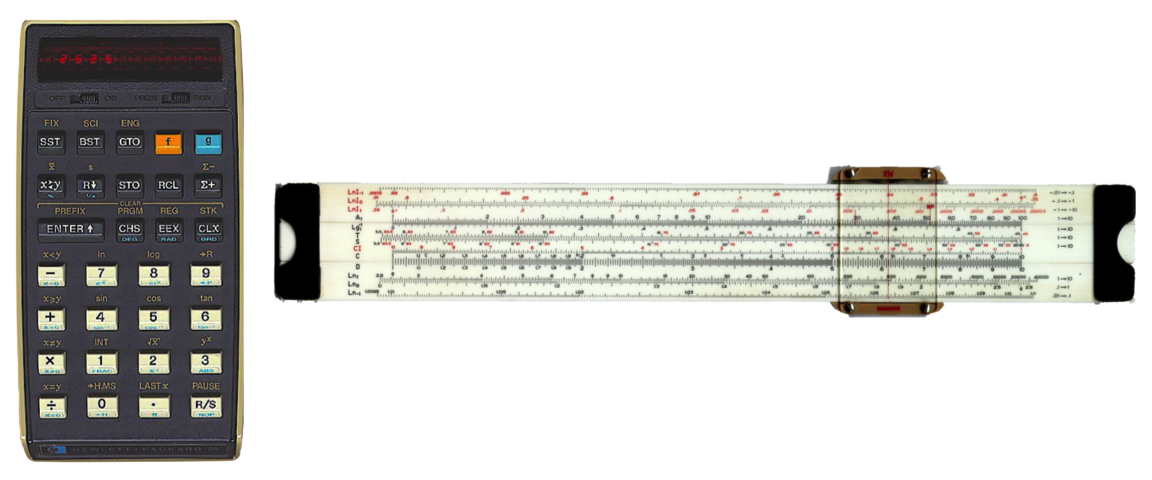 Left: the venerable HP-25 programable (!) scientific calculator. Right: a slide rule used for all calculations until the early 1970’s. It was not programmable (although it was wireless)
Today I’ve got more processing power in my watch then I had in that calculator. But I’ll bet you’ve got something like it…calculators are nothing but electronic function machines. In fact, this is the arithmetic circuit inside of that original calculator:
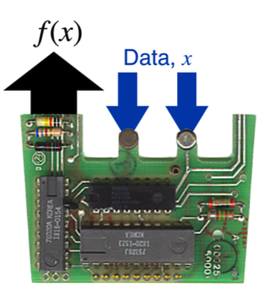
The calculator guts shows what a function does: if you enter data through the keypad—a value of $x$—and hit the appropriate button, the display shows the value of the function. So if the function was the formula $f(x) = x^2$ and if I keyed in “4” and pushed the $x^2$ button, the display would read “16,” the value of $f(4)$ for that particular function. Notice that it doesn’t give you more than one result, and that’s a requirement of a function: one result.
That’s all a function is: a little mathematical machine that reports a single result for one or more inputs according to some rule. For us, functions can be represented by a formula, an algorithm, a table, or a graph. In all cases, it’s one or more variables $x$ or $x \; \& \; y…$ or $x \; \& y \; \& z…$ in, a rule about what happens to them, and one numerical result out.
Nature seems to live by functions and since we’re all about nature, we’ll need to use functions. Our way.
Turn the crank, QS&BB style
We’ll accomplish a lot without much mathematical effort, I promise you. In fact, we’ll find that the raw mathematics of modern physics is simple. What’s hard is the conceptual visualization.
Don’t fear the math! Your adversary will be your hard-wired common sense!
Some physics models are simple and we can easily deal with them in their “raw” mathematical form…and some are really quite complicated. With a little help from Mr Descartes or some whimsy, we’ll manage. So three ways we’ll work with mathematical models.
1. We’ll write them and manipulate them for real.
Can you solve the equation: $y = ax$ for $x$? You’ll be surprised just how often an equation of that form will describe sophisticated aspects of the world.
2. Plot them.
If I want to deal with a model that uses sophisticated mathematics quantitatively, instead of working with the formulas…I’ll just show you the functions are plotted. Here’s an example, a really important model in physics which we’ll refer to a number of times. The function is messy and I don’t want to lose track of the physics by getting you bogged down in evaluating the it.
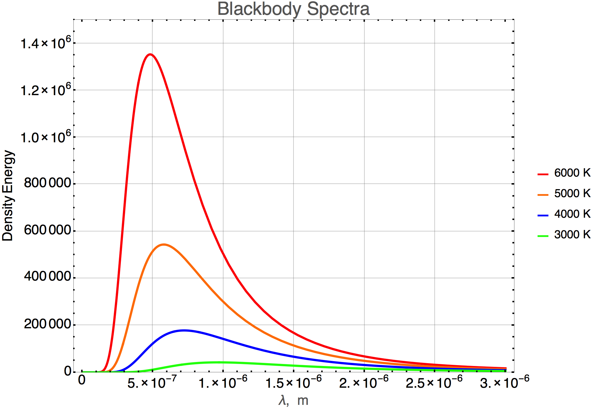 This is the intensity of a heated object as a function of wavelength of the radiation for different temperatures.
You’d have no problem telling me the relative intensities of say the blue and the red curves—4000 degrees and 6000 degrees—at a wavelength of 1 micron, $1 \times 10^{-6}$ m. Right? Much easier than plugging into Mr Planck’s formula.
3. Represent with a circuit. A silly circuit.
If we’re talking about a really complicated model, perhaps one with many formulas and lots of high-brow calculus or even worse, I’ll show you a cartoon and ask you to take my word for it.
Remember in your past you might have heard someone use the phrase, “turn the crank…” that’s sort of old language for plugging in some numbers and doing some laborious calculation…. We’ll not do that. I’ll just show you this figure, properly filled out for the circumstance at hand:
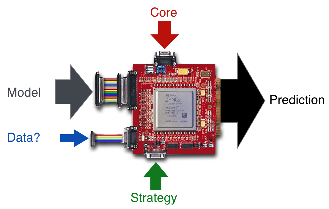 The evaluation of a candidate physical model (which is a function or a set of functions) requires some inputs [the equation(s), maybe some data, some core beliefs (other trusted models),and some plan…a strategy]. The result is a prediction which would almost always be a prediction for some measurable quantity.
What will be important here is that we all agree on the assumptions in the model, the tools used to solve it, and any data that might be a part of the calculation of interest. You’d have no problem imagining a computer solving something or running some (game?) simulation and that’s all this fake circuit represents. Something in, some instructions, and something out. We move on.
A Gentle Review 1: Skills You’ll Frequently Need
You might find it useful to brush off some previous skills that we’ll need to make progress. I have in mind simple algebra, exponents, powers of 10, and some simple geometry formulas.
Some Algebra Practice
I’ll show you some examples of the level of algebra we’ll need, but let’s first pause and salute the most important thing about algebra:
The Fairness Doctrine of Algebra: If you do something to one side of an equation, you must do the same thing to the other side.
Words to live by. Armed with this, here we go. You’ll be surprised how simple this will be.
Our appetite for algebraic complexity will be very modest. We’ll not encounter formulas that are much more complicated than these:
(Were you writing? I’ll wait.)
Can you do each of these? Then you’re good: that’s about all that you’ll need to remember of algebra. Just remember the rule. Then…it’s merely a game—a puzzle to solve.
The Powers That Be: Exponents
Once in a while, we’ll need to multiply or divide terms that have eyponents. There are simple rules for this, but let’s figure them out by hand…so to speak. The first thing to remember about exponents is that in a term like $y^n$, a positive integer $n$ tells you how many times you must multiply $y$ by itself. So: $y^1 = y .$ Here, there’s just one $y$, so: $y^1 = y.$
Suppose I have $y\times y$ You’d be pretty comfortable calling that “y-squared” and from the above, the number of $y's$ there are in that product is two. So $y\times y = y^2.$ If I add another product, then I’d have $y\times y \times y = y^3.$ Get it? Notice that what we’ve also got in this equation is: $y\times y \times y = y^2 \times y^1= y^3$ and we’ve just developed our first rule on combining exponents:
$y^n \times y^m = y^{n+m}.$ Now you try it.
An Example: Exponents together
The Question: What is $x^2x^1x^4$ ?
$x^2x^1x^4=x^{2+1+4}=x^{7}$
Interactive: 3.1; 2018.10.15; 17:06 Exponents, you do it
One more time, but different. Another rule recalling that a negative power means “one over…”:
$x^{-n} = \frac{1}{x^n}.$
If the same rule for adding exponents works—and it does—then we can multiply factors with powers by keeping track of the positive and negative signs of the exponents.
So here’s an easy one: $\frac{x\times x \times x}{x\times x} = x$ which you quickly get by crossing out two $x$’s in the numerator and the denominator leaving you with one left over.
Or, by using the powers and the rule:
Interactive: 3.2; 2018.10.17; 14:31 What is $x^{−2}x^1x^4$?
One more thing. The powers don’t have to be integers.
Perhaps you’ll remember that square roots can be written:
That’s it. Now we have everything we need to turn numbers into sizes of…stuff.
The Big 10: “Powers Of 10,” That Is
One of the more difficult things for us to get our heads around will be the sizes of things, the speeds of things, and the masses of things that fill the pages of QS&BB. Lots and lots of zeros for a large or small number means: lots of mistakes and a hopelessness for the relative magnitudes of one big or small thing compared to another. Big and small numbers are really difficult to process for all of us.
I have no idea how much bigger is the Milky Way Galaxy (950,000,000,000,000,000,000 meters) than the diameter of Jupiter (143,000,000 meters). It all blends together.
Wait. That sounds pretty grim.
Glad you asked. But wait. There’s a solution: the beauty of “10” or lots of “10’s.”
Exponential notation…using our power rules and the number 10. It’s easy.
A number expressed in exponential notation as:
Let’s think about this in two parts. First, the 10-power part.
The rules above work for 10 just like any number, so $10^n$ is shorthand for the number that you get when you multiply 10 by itself $n$ times. This has benefits because of the features of 10-multiples, that we count in base-10, and now you can just count zeros. So for example:
The power counts the zeros, or more specifically, the position to the right of the decimal point from 1. So if you have any number, you can multiply it by the 10-power part and have a compact way of representing big and small numbers.
The second thing is the number in front that multiplies the power of 10. It’s called the “mantissa” and that’s all it is…a number.
The powers of 10 come with handy nicknames that imply a particular amount… like “kilo-gram,” meaning 1,000 grams. You already know many of them. Here are more powers of 10 than you ever want to know:
| nickname | prefix | symbol | factor | power of ten |
|---|---|---|---|---|
| septillionth | yocto- | y | 0.000000000000000000000001 | $10^{-24}$ |
| sextillionth | zepto- | z | 0.000000000000000000001 | $10^{-21}$ |
| quintillionth | atto- | a | 0.000000000000000001 | $10^{-18}$ |
| quadrillionth | femto- | f | 0.000000000000001 | $10^{-15}$ |
| trillionth | pico- | p | 0.000000000001 | $10^{-12}$ |
| billionth | nano- | n | 0.000000001 | $10^{-9}$ |
| millionth | micro- | $\mu$ | 0.000001 | $10^{-6}$ |
| thousandth | milli- | m | 0.001 | $10^{-3}$ |
| hundredth | centi- | c | 0.01 | $10^{-2}$ |
| tenth | deci- | d | 0.1 | $10^{-1}$ |
| one | 1 | $10^{0}$ | ||
| ten | deca- | da | 10 | $10^{1}$ |
| hundred | hecto- | h | 100 | $10^{2}$ |
| thousand | kilo- | k | 1,000 | $10^{3}$ |
| million | mega- | M | 1,000,000 | $10^{6}$ |
| billion | giga- | G | 1,000,000,000 | $10^{9}$ |
| trillion | tera- | T | 1,000,000,000,000 | $10^{12}$ |
| quadrillion | peta- | P | 1,000,000,000,000,000 | $10^{15}$ |
| quintillion | exa- | E | 1,000,000,000,000,000,000 | $10^{18}$ |
| sextillion | zetta- | Z | 1,000,000,000,000,000,000,000 | $10^{21}$ |
| septillion | yotta- | Y | 1,000,000,000,000,000,000,000,000 | $10^{24}$ |
A “feel” for sizes is pretty much limited to our puny human experiences. I can probably estimate a length of about 10 feet. So I might be able to approximate the hight of a building, for example. Or compare the distances of two plots of land. But much more than that, I’m out of in-grained tools. Well, this is “particle physics” and “cosmology”…the smallest items and the largest ones in the whole universe. So the prefixes in the list above? We’ll need many of them. Here’s a list of “things” from normal to, well, extreme.
The Big and the Small of QS&BB: Sizes in the Universe
Here is a ranked list of big and small things with approximate sizes, along with the nicknames that we use. We’ll span these enormous distance ranges and eventually Tera-this and pico-that will just roll off your tongue.
Big Stuff
- African elephant, 4 m
- Height of a six story hotel, 30 m, $3.0 \times 10^1$ m
- Statue of Liberty, 90 m, $9.0 \times 10^1$ m
- Height of Great Pyramid of Giza, 140 m, $1.4 \times 10^2$ m
- Eiffel Tower, 300 m, $3.0 \times 10^2$ m
- Mount Rushmore 1700 m, $1.7 \times 10^3$ m, 1.7 km
- District of Columbia, 16,000 m square, $16.0 \times 10^3$ m, or $1.6 \times 10^4$ m
- Texas, East to West, 1,244,000 m, $1.244 \times 10^6$ m, 1244 km, or 1.244 mega-m
- Pluto, 2,300,000 m diameter, $2.3 \times 10^6$ m
- Moon, 3,500,000 m diameter, $3.5 \times 10^6$ m
- Earth, 12,800,000 m diameter, $12.8 \times 10^6$ m, or $1.28 \times 10^7$ m
- Jupiter, 143,000,000 m diameter, $143.0 \times 10^6$ m, or $1.43 \times 10^8$ m
- Distance Earth to Moon, 384,000,000 m, $384.0 \times 10^6$ m, or $3.84 \times 10^8$ m
- Sun, 1,390,000,000 m diameter, $1.39 \times 10^9$ m, 1.39 giga-m
- Distance, Sun to Pluto, 5,900,000,000,000 m, $5.9 \times 10^{12}$ m, 5.9 tera-m
- Distance to nearest star (Alpha Centuri), 41,300,000,000,000,000,000 m, $41.3 \times 10^{18}$ m, or $4.13 \times 10^{19}$ m, 41.3 Exa-m
- Diameter of the Milky Way Galaxy, 950,000,000,000,000,000,000 m, $950 \times 10^{18}$ m, or $9.5 \times 10^{19}$ m, 9.5 Exa-m
- Distance to the Andromeda Galaxy, 24,000,000,000,000,000,000,000 m, $24.0 \times 10^{21}$ m, or $2.4 \times 10^{22}$ m, 24 zetta-m
- Size of the Pisces–Cetus Supercluster Complex, our supercluster, 9,000,000,000,000,000,000,000,000 m, $9.0 \times 10^{24}$ m, 9 zetta-m*
- Distance to UDFj-39546284, the furthest object observed, 120,000,000,000,000,000,000,000,000 m, $120 \times 10^{24}$ m or $1.2 \times 10^{26}$ m
* This is out of hand. we have different units for astronomical objects!
Small Stuff
- Circumference of a basketball, (regulation 30 inches) 0.762 m, 76.2 cm
- Diameter of a golf ball, 0.043 m, 4.3 cm, or 0.043 m, 43 milli-m, mm
- Diameter of a green pea, 0.001 m, 1 cm, or 0.01 m, 10 mm
- A small ladybug, 0.5 cm, 0.005 m or $5\times 10^{-3}$m, 5 mm
- A human hair diameter. $10^{-4}$ m, 100 $ \text{micro-m, } 100 \mu$m
- Wavelength of mid infrared wave, $100 \times 10^{-6}$ m, $100 \mu$m
- A human cell. $10^{-6}$ m, 10 $\mu$m
- A large molecule. Sugar, $6 \times 10^{-10}$m, 0.6 nm, 600 pico-m, pm
- A large atom. Cesium atom (largest) $ 2.225 \times 10^{-10}$ m, 0.225 nm, 225 pm
- Wavelength of soft X-ray (12.4 keV), $100 \times 10^{-12}$ m, 100 pm
- Wavelength of hard X-ray (124 keV, 300 EHz), $10 \times 10^{-12}$ m, 10 pm
- Compton wavelength of an electron, $2.4 \times 10^{-12}$ m, 2.4 pm
- Bohr radius, $53 \times 10^{-11}$ m, 53 pm
- 1 Angstrom, $10^{-10}$ m, 100 pm
- Radius of Helium nucleus (alpha particle). $1.6 \times 10^{-15}$m, 0.016 femto-m, fm
- Radius of a gold nucleus. $7 \times 10^{-15}$ m, 0.000007 nm, 7 fm
- A hydrogen nucleus (a proton). $ 1.3 \times 10^{-15}$ m, 0.0000013 nm , 1.3 fm
- Radius of a quark (upper limit), $10^{-18}$ m, 1 am
- The smallest distance that can exist: the “Planck length,” $10^{-35}$ m
I don’t know Mr Huang, but his Scale of the Universe 2 (http://htwins.net) is worth playing with, if not owning his app. You know. For parties.
Geometry, curves…Formulas From Your Past?
We will deal with some functions that would be very hard to evaluate on your calculator. But Descartes’ gift is that I can show you the graph and evaluation can be done by eye, which is in effect solving the equation. We’ll use some simple geometrical relations which I’ll summarize here.
Formulas from your past that might be explicitly useful
I know that you’ve seen most of this somewhere in your past! So return with us now to those thrilling days of yesteryear. Straight lines, circles, and the areas and circumference of circles and triangles are useful.
Equation of a straight line
A straight line with a slope of $m$ and a $y$ intercept of $b$ is generally described by the equation,
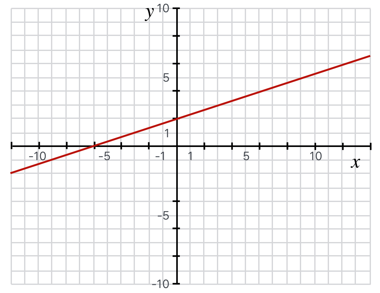 A straight line with a slope of $1/3$ and a $y$ intercept of $2$, so $y=1/3x+2$.
Equation of a circle
A circle of radius $R$ in the $x-y$ plane centered at a $(a,b)$ is described by the equation:
Of course if the circle is centered at the origin, then it looks more familiar as in this figure:
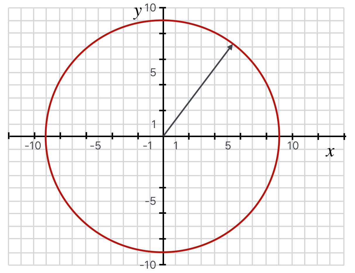 A circle centered at the origin described by the equation, $x^2 + y^2 = 81$. It has radius of $9$, area $A=\pi 9^2$, and circumference $C=2 \pi 9.$
Equation of a parabola
A parabola in the $x-y$ plane facing up with vertex at $(a,b)$ where $C$ is a constant has the equation,
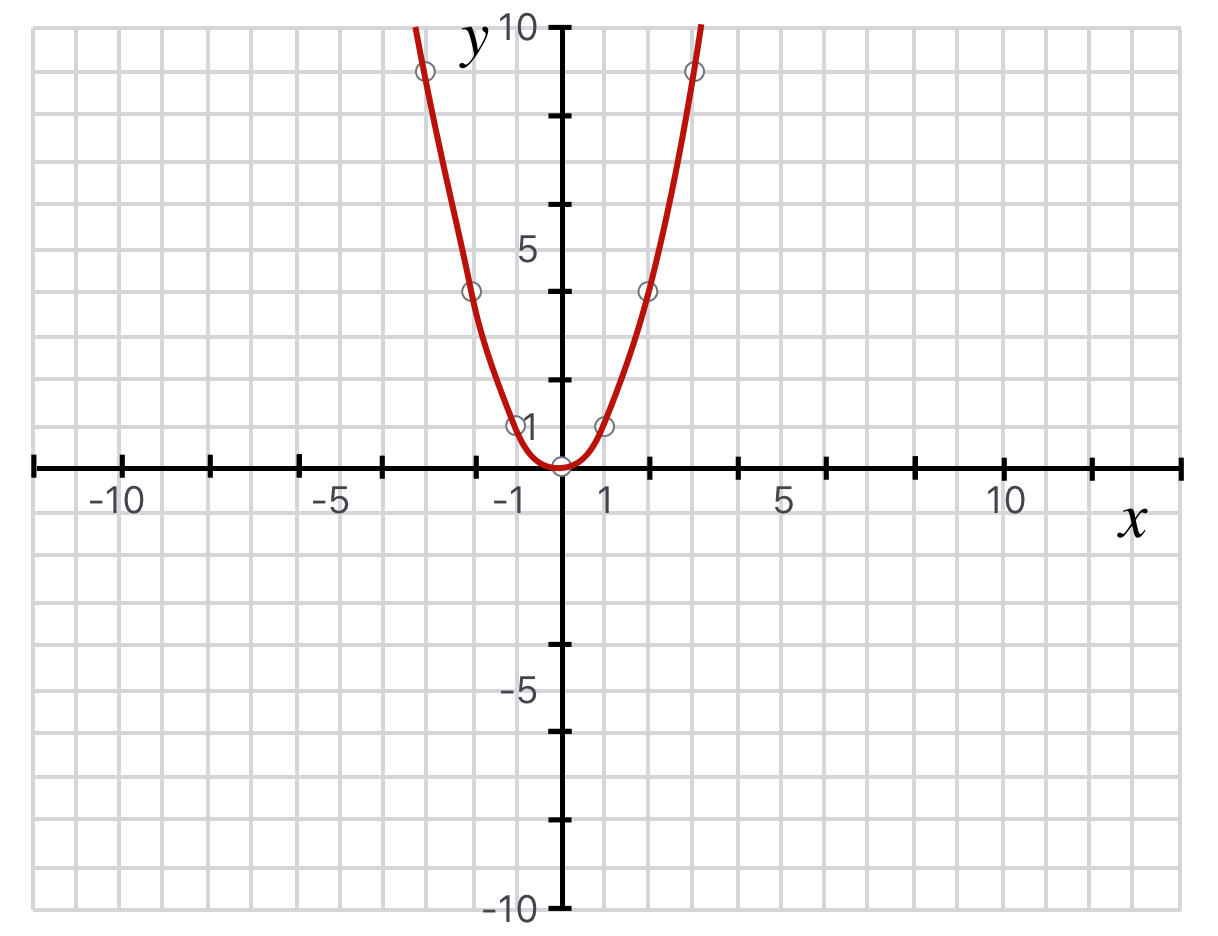 A parabola satisfying the equation, $y = 1x^2$.
Area of a rectangle
A rectangle with sides $a$ and $b$ has an area, $A$ of
Area of a right triangle
A right triangle (which means that one of the angles is $90$ degrees) with base of $a$ and height of $b$ has an area, $A$ of
For a right triangle, the base and height are equal to the two legs. But the formula works for any triangle. Here are some examples,
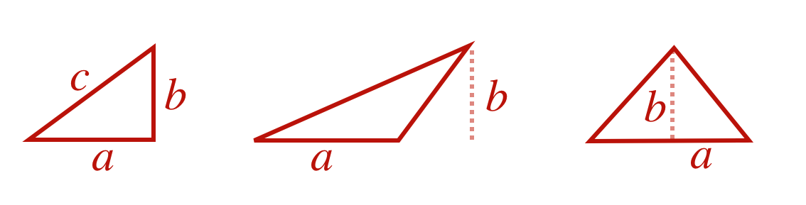 Three triangles, all with the same areas.
Area and circumference of a circle
For a circle of radius $R$, the area, $A$ is
and the circumference, $C$ is
Pythagoras’ Theorem
For a right triangle (like the left hand triangle above), the hypotenuse, $c$ is related to the lengths of the two sides $a$ and $b$ by the Theorem of Pythagoras:
And, no. He didn’t invent it and it’s been proven many, many different ways.
The quadratic formula
We might run across a particular polynomial, which you’ve also probably seen before:
It’s an “order 2” polynomial, which means that there are two values of $x$ that qualify as “solutions”: the values of $x$ that when substituted make the function be zero. You could plot the function and find what $x$ values the curve passes through the $x-$axis, or you could rely on the time-honored recipe:
A Gentle Review 2: Skills for Only a Few Times
There are a handful of skills that will sometimes come up, but not every lesson. I have in mind here reading log-plots, unit conversions, approximating functions, simple graphical vector manipulations, and a few more geometrical relationships.
Log-Log and Semi-Log Plots
Wait. LOGARITHMS!!? NO!
Glad you asked. Calm down. There will be only a couple of times when I’ll ask you to read a plot…meaning identify a point on a curve in which the axes are not linear (1, 2, 3, 4…) but logarithmic (10, 100, 1000…). No functional manipulations. Just interpretation.
Sometimes it will be useful to plot functions or data that range over a wide scale, maybe even many powers of 10. I want to make use of log-log plots and semi-log plots because it’s about the only way to display functions that range over many orders of magnitude. So we’ll use them as a tool, but we’ll never actually evaluate a logarithm. Here’s an example.
We’ll learn that there is a relationship between the time it takes for a planet to orbit the sun (its “period”) and the distance away that its orbit is from the center of the sun. Here it is for a slice of distances. The graph displace orbital period in units of days versus the distance from the sun in units of 100,000,000 kilometers. So the left hand “origin” is at 100,000 km, then the next big tick mark is at 110,000,000 km and the next (labeled) tick mark is at 120,000,000 km. That’s a lot of zeros, so I labeled the horizontal axis as units of $10^8$ km.
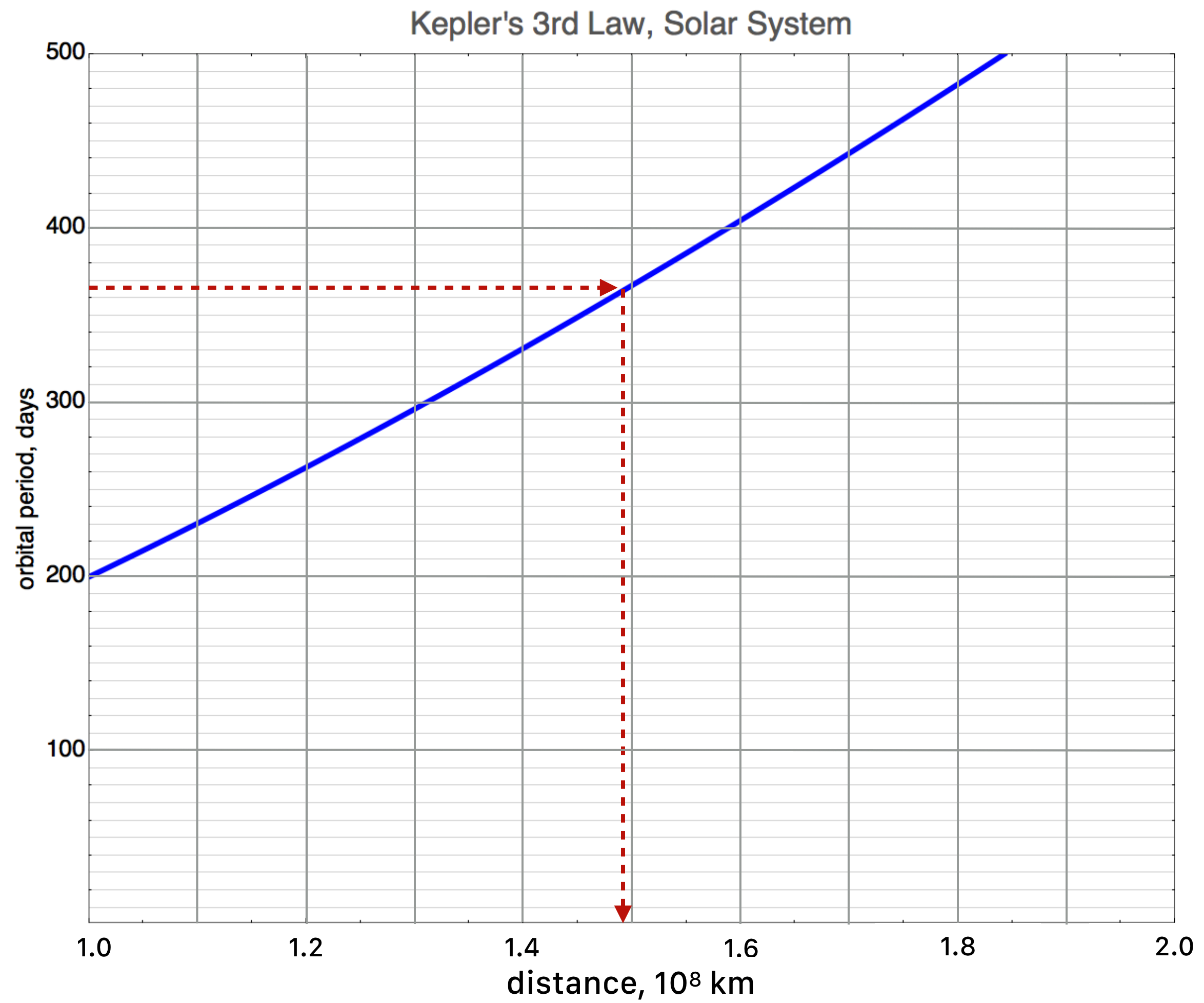
If I asked you to find the distance earth, which has a period of 365 days, is from the sun, you’d look at the vertical, period axis, dig into the tick marks, and figure out where to find 365 on the vertical axis, right? I’ve kind of done that—what your finger would probably do—and I find that the horizontal, light lines are at every 10 days and the tick marks are at every 20 days, so I’d find 365 at about where the horizontal arrow is. Using the model—solving the equation that relates period to distance—means simply finding the point on the curve and reading down to the distance. Going down from the curve, it would hit at about $1.5 \times 10^8$ km. That’s about right.
If I asked you to do the same thing for Venus, but the other way around you could do that:
Interactive: 3.3; 2018.10.19; 13:41 d=1.07e8km -> 226 days
How about Mars? Its period is about 687 days. Certainly the model (the blue line) should describe Mars. How about Mercury? Its period is 87 days and it’s distance is $0.58 ]\times 10^8$ km. How about Neptune? It’s period and distance are 60,200 days and $44.8\times 10^8$ km. None of these fit on the graph. So this plot is pretty useless as a guide to the solar system. Don’t despair. There’s a way.
This is where a log-linear or log-log plot saves the day. In a log plot the axes are labeled by powers of 10, so 1, 2, 3… and so on, standing for $10^1, 10^2, 10^3$. This power relation distorts the curve from presentation on a linear scale pair, but it’s not wrong, just different. Let’s do that for our solar system for the horizontal axis.
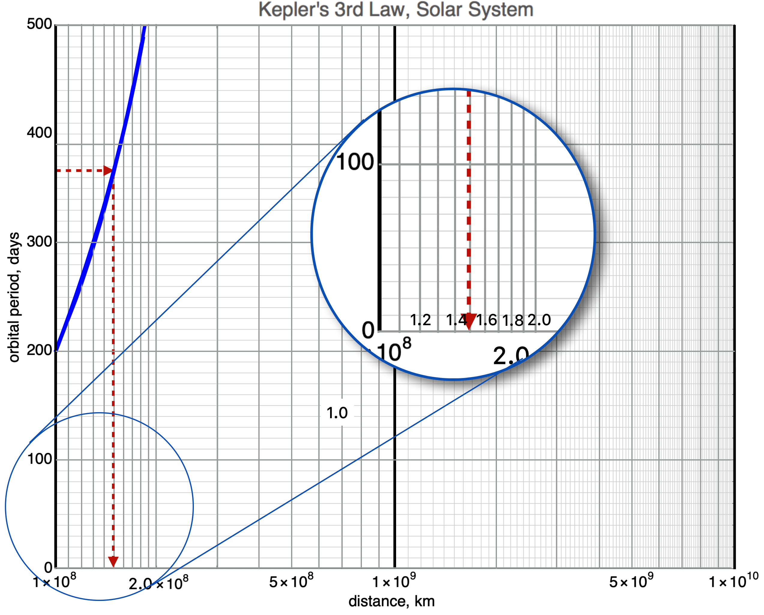
In this figure, the dark, black vertical lines tell you the $1\times 10^8, 1\times 10^9, \text{ and } 1\times 10^{10}$ km marks. The vertical gray lines indicate the $ 2,3,4,5,6,7,8,9\times 10^{8,9,\text{ or }10}$ km marks. The circular inset breaks down the $10^8$ region to that of the linear horizontal plot up above. Notice that the red, dashed lines mean what they did in the first plot: 365 days for Earth’s period on the vertical axis and about $1.5 \times 10^8$ km for Earth’s distance from the center of the sun on the horizontal axis.
But we still can’t represent much of the solar system in one plot, so we must also make the vertical axis logarithmic. A “log-log” plot, whereas the previous is a “linear-log” or “semi-log” plot. Here it is, the model of orbiting planets around our particular Sun. Earth is again represented as the red, dashed lines and now we can evaluate the periods and distances for many more planets.
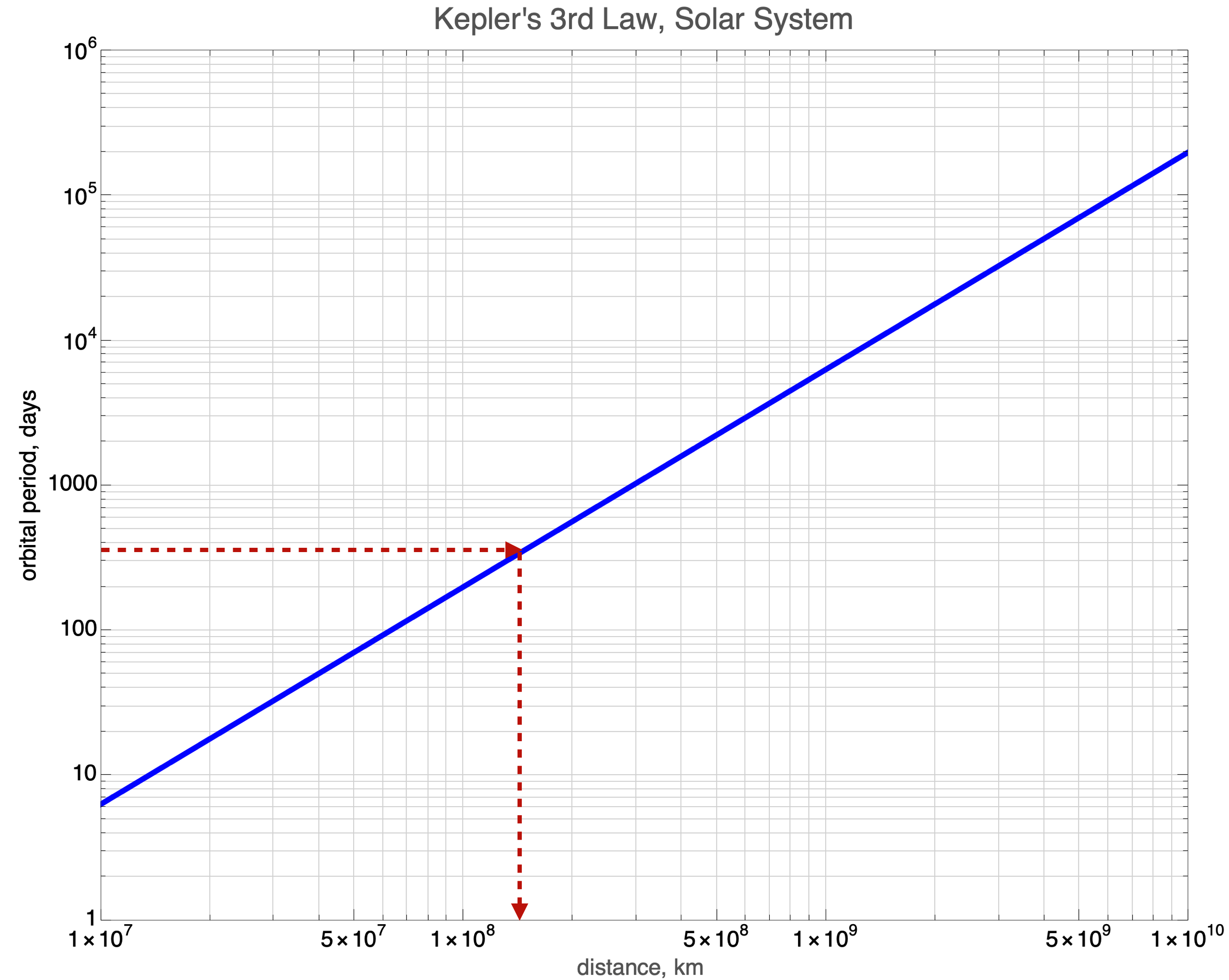
This covers 6 orders of magnitude in days and 4 orders of magnitude in kilometers.
Interactive: 3.4; 2018.10.23; 16:04 The planet jupiter is 778.5 million miles from the sun. What is its period (jupiter’s “year”) in days?
Unit Conversions
Numbers are just numbers without some label that tells you what they refer to. Not all numbers have to refer to something, a pure number is a respectable mathematical object—prime numbers for example have been a topic of research for centuries. Irrational numbers—those that can’t be expressed as a ratio of whole numbers, like $\pi$, —are likewise objects with no necessary relationship to…“stuff” in our world. But they keep coming up in nature, so we warm to them.
We’re mostly concerned with numbers that measure a parameter or count physical things and they come with some reference unit (“foot”) that is a customary way to compare one thing with another. Of course not everyone agrees on the units that should be used. Wait. Let me restate that: there’s THE WHOLE WORLD that agrees on one set and then there’s the United States that marches to its own set of units. Thinking of you, “feet,” “pounds,” and “Fahrenheit.”
I’ll not use Imperial units (feet, inches, pounds, etc.) very much, except to give you a feeling for something that you’ve got an instinct for…like the average height of a person or a single story house. We’ll use the metric system, in particular the MKS, aka SI units1 in which the fundamental length unit is the meter (about a yard), the fundamental mass unit is the kilogram, and the fundamental temperature unit is the Celsius. I’ll generically refer to these as “MKS” (for meter-kilogram-second) or “metric units” without being too fussy about the fancier names, like SI.
It’s small comfort that we’re all in agreement on seconds, minutes, and hours and its base-60 origins. In 1793 the French tried to change that to “decimal time” with a 10-hour day, 100 minutes in an hour, and 100 seconds in a minute and so on, but it didn’t catch on.
Just like an exchange rate in currency, so many euros per dollar, we’ll need to be able to convert, among many different units. All the time.
Wait. That can be pretty involved.
Glad you asked. You’re right and it can be a way to make mistakes and get all wrapped up in the conversion that you lose track of the physics. You know what? I’ll not care. I’ll give you little conversion engines that will do any unit conversion that you need to do. Just let me show you what it means and then we’ll be pretty low-key about this.
Having said that, we should review how this works—what will be behind any tool that does unit conversion.
Let’s get our bearings. What’s the height of an average male. Mr Google tells me that’s about 5’10”. How many inches tall is our average male? Here’s the pre-QS&BB thought-process you’d use to calculate this.
Three steps:
- A single foot is $12$ inches.
- So, $5$ feet is $5 \times 12$ = $60$ inches
- and the combination is $60 + 10 = 70$ inches.
…which you could almost do in your head, which, by the way, averages in circumference at about 22 inches. You’re welcome.
But this simple, almost intuitive calculation uses a more general conversion from one unit to another through a tricky multiplication by the number 1. Can you multiply by 1? Then you can convert units like a champ.
While this is a particularly simple conversion, sometimes we’ll need to do some which are either more complicated, or use units that maybe you’re not very familiar with. I won’t be so pedantic usually, but hopefully you get the point!
Let’s work out an example. Something you can use at a party. I first worked this out for a class when I was in Geneva, Switzerland working at CERN. It was July 4, 2010, which was just another Sunday over there. The United States came into existence on July 4, 17762 which was $2010-1776 = 234$ years ago.
fireworks
How many seconds had the United States been around if we start from midnight on July 4, 1776?
We need a handful of 1’s here:
Now it’s a matter of just multiplying by the right combinations of “1” as many times as necessary to get where you want to be.
There are a few of things to notice here. First, that’s a lot of seconds! Second (get it?), if we’d known that there are $3.154 \times 10^7$ seconds in a year we could have started with that and had just one factor of 1. And finally…“3.154”? Does that sound familiar to anyone?
Quite by accident, the number of seconds in a year is close to the first few digits of $\pi = 3.14159…$ times $10^7$ and so we often say that the number of seconds in a year is about “$\pi \times 10^7$.”
Just as a memory device. You’re welcome.
Vectors
Some quantities in nature have a magnitude (like a temperature) and a magnitude and a direction, like a velocity. 60 mph north does not result in the same trip as 60 mph east, so direction and speed both matter. I think that the most intuitive vectors are those associated with a distance in space and a force, so in this survey I’ll concentrate on those two. We’ll meet many other vectors throughout QS&BB, but I’ll highlight their vector natures when we come to them. As I’m writing this, the World Series in 2018 is about to start, so let’s think about a baseball diamond.
In baseball, the distance between the bases is 90 feet and according to the rules, a runner must follow the bases in order. So to go from home plate to second base, the path that’s followed must be according to the two arrows in this figure. This situation is shown in the (a) below. Here, Frank has hit a double and being a good sport has indeed taken the appropriate path to second base.
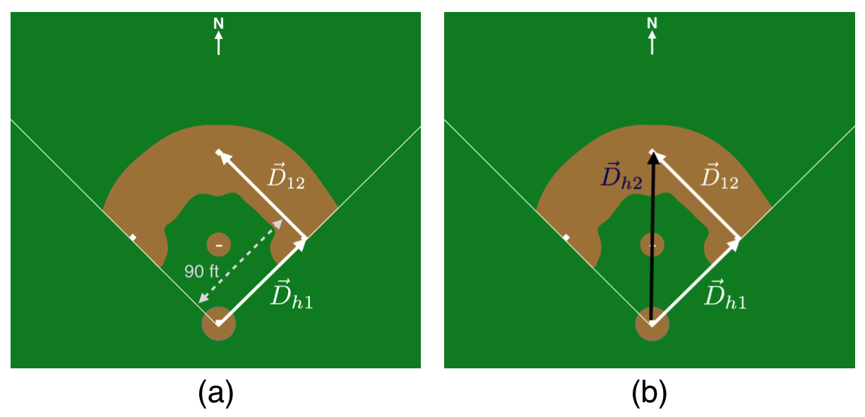 Figure (a) shows the appropriate path to second base. (b) Shows an illegal path to second base.
In order to represent all of the information in a vector, we'll be satisfied with either a graphical representation---a labeled picture---or something else. Here's an example. If Ossie hits a single, we could represent his trajectory vector from home to first base as $$\vec{D}_{h1} = 90 \text{ ft NE}. \nonumber$$ The formal name for a vector in regular space is *displacement* and the formal name for the magnitude of a displacement vector is *length* or *distance* so the vector $\vec{D}$ is the displacement and 90 ft is the length. Maybe not the way you might have seen a vector displayed, but it's perfectly okay. It encodes the length (90 feet) and the direction (northeast) in one thing. Next up, Dewey smacks a double, and so his vector would be $$\vec{D}_{h1} + \vec{D}_{12}. \nonumber$$ Chester is up next and realizes that the *shorter distance* from home plate to second base is straight north across the diamond over the pitcher's mound, which is shown in (b). While he hit the ball to the warning track, after that day he didn't play long on that team since he took that shorter path and was called out for not following the rules. What's okay in mathematics is not necessarily okay in baseball. Chester is right, though. Before he was called out, he correctly navigated what is actually the vector sum of two vectors: $$\vec{D}_{h2 } = \vec{D}_{h1} + \vec{D}_{12}. \nonumber$$ Both the left hand and the right hand of that equation are equivalent in that they both connect home plate with second base.
falling down
Earlier Earl was at bat and hit a ground ball to the shortstop but he fell down halfway to first base. How does his displacement compare to Ossie’s in vector notation?
Before his embarrassment, Earl was running in the same direction that Ossie ran—and thousands of ball-players before them. However his vector would be:
an arrow pointing from home plate halfway to first base.
Interactive: 3.5; 2018.10.23; 16:51 Dewey was also unlucky and after Chester was called out he tried to steal third base from second base, but fell down 1/3 of the way. What’s the vector that represents his short trip?
In QS&BB we’ll make a lot of use of the handy arrow symbol: $\rightarrow$. The length of the arrow represents the magnitude and of course the orientation and the head of the arrow represent the direction. Arrows can be $\longrightarrow$, or short $\rightarrow$, pointed in different directions, $\nwarrow$, $\leftarrow$, $\nearrow$, etc. Very handy.
The magnitude can mean many things, depending on the physical quantity being represented. Some of the vectors that we’ll meet are displacement, velocity, momentum, force, electric field, magnetic field, and angular momentum.
A few useful things from this figure:
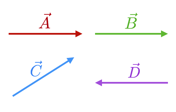 Random vectors, all of the same length.
Two vectors, $\vec{A}$ and $\vec{B}$ are said to be equal if they are both the same length and point in the same direction so
Vector $\vec{C}$ is the same length as both $\vec{A}$ and $\vec{B}$ but
because its direction is different. Finally, the negative of a vector is that same vector pointing in the opposite direction. So for example,
Vector addition
Generally, we’ll treat a vector quantity as an arrow pointing in some direction and a length that represents its magnitude. Sometimes a vector can represent an actual path in space (like meters, feet, and so on) where it’s easy to imagine what it means. We do this all the time on maps with a scale showing that some map-distance (an inch) can stand for a real-world distance (“1 inch = 1 mile”).
But, sometimes a vector doesn’t represent a length in space, but some other physical quantity, like a force or a velocity. This can be complicated since you’re drawing an arrow that has a “regular” length, but you mean it to be something else, like a force. But, it still works geometrically (the arrow still points in space) and we just use a different scale. Let’s do something simple.
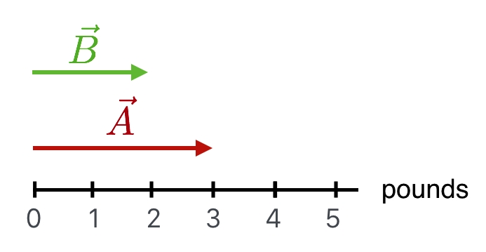
If $\vec{A}$ corresponds to Muriel pulling the leash on her reluctant and enormous dog and vector $\vec{B}$ corresponds to Earl's ability to also pull, then the two of them together can pull with the obvious 5 pounds.
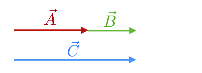
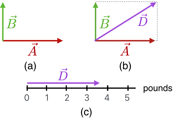
Here’s a different combination of vectors, which looks more like Chester’s baseball career’s embarrassing final act. Here, we have two vectors that have the same lengths on your screen, but now their lengths represent displacement (both a distance and a direction). They look like the force vectors and their lengths on your screen are the same, but the units are different: $\vec{A}=3$ blocks and $\vec{B}=2$ blocks.
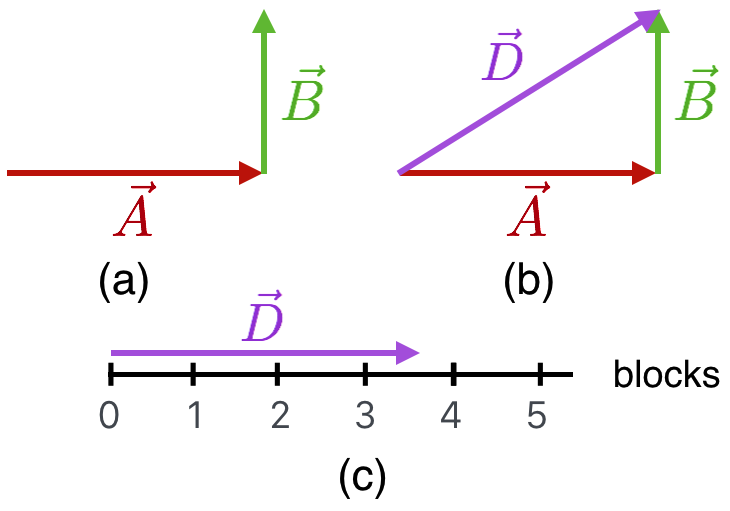
This situation represents a trip through city blocks on the sidewalk: (a) going east $\vec{A}$ and then north, $\vec{B}$. Equivalently, (b) represents a trip from the same starting point to the same ending point by cutting across a park, $\vec{D}$. That third vector is gotten by doing the same tail-to-head manipulation as we did in one dimension. Of course, you'd create that third vector by just walking straight across the park. $\vec{D}$ is equivalent to the combination of $\vec{A}$ and $\vec{B}$, which is to say $$\vec{A} + \vec{B} = \vec{D}$$ Obviously, it's useful to figure out whether the diagonal path is shorter than the sidewalk paths (thats' clear by looking) and just how much shorter it is. For that, we need the scale. Let's use the standard notation that the length (or "magnitude") of a vector is $\lvert\vec{V}\rvert$. So here $\lvert\vec{A}\rvert = 3$ blocks and $\lvert\vec{B}\rvert = 2$ blocks.
get off my lawn
In the figure, how much shorter is cutting across the park as compared to traveling on the sidewalk?
Obviously the sidewalk journey is $3 + 2 = 5$ blocks. What’s the length of $\vec{D}$? We can do this two ways. One way is to look at the triangle in (b) and remember Pythagoras’ Theorem.
Or we can use the scale, as in (c)…construct $\vec{D}$ with the head-tail rule and then just transplant it to the scale and see that its length is indeed a little more than 3 and a half. Or, somehow move the scale like a ruler and measure the length of $\vec{D}$.
Either way, it’s shorter to cut across the park by almost a block and a half. But you sort of knew that.
Here’s another situation.
So their total pull here is going to be less than 5 pounds and will be some total amount that's oriented between the two. The (b) figure shows another way to add vectors as a manipulation. Instead of tail to head, (b) shows a placeholder parallelogram drawn in dashed outline and the sum of the two vectors is the diagonal. Of course it's the same vector you'd get if you'd transported $\vec{B}$ horizontally to the head of $\vec{A}$ and added them as before. So this is actually an alternative way to construct vectors sums: the head-to-tail way or the parallelogram way.
An inverse of the process of adding two vectors is called resolving or decomposing a vector into its components. This figure shows the steps and is literally the parallelogram addition-method done backwards!
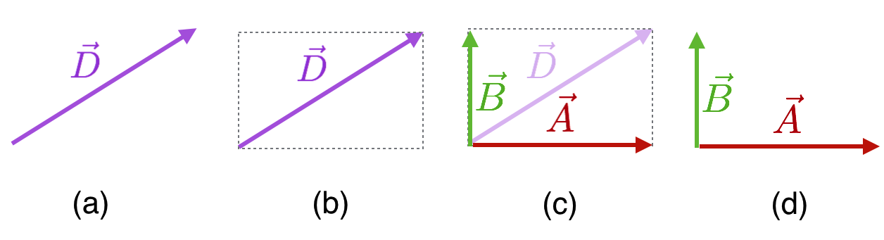 The successive steps involved in “resolving” a vector into its perpendicular components.
Let’s decompose vector $\vec{D}$ into components along the horizontal and vertical directions (it could be any two directions and they need not be perpendicular). The way to construct this is to add a placeholder parallelogram — usually a rectangle — with the original vector across a diagonal. Then the sides become the two decompositions: the vector components. In both of these cases we’re doing:
Here going from left to right (decomposition of $\vec{D}$) and just before, going from right to left (addition of $\vec{A} \text{ and } \vec{B}$).
We absorb the subtraction sign into the direction designation of $\vec{D}$ and make a new vector, $\vec{E} = -\vec{D}.$...and then add them. This shows the whole sequence of $\vec{A}-\vec{B} = \vec{A} + \vec{E} = \vec{D}$:
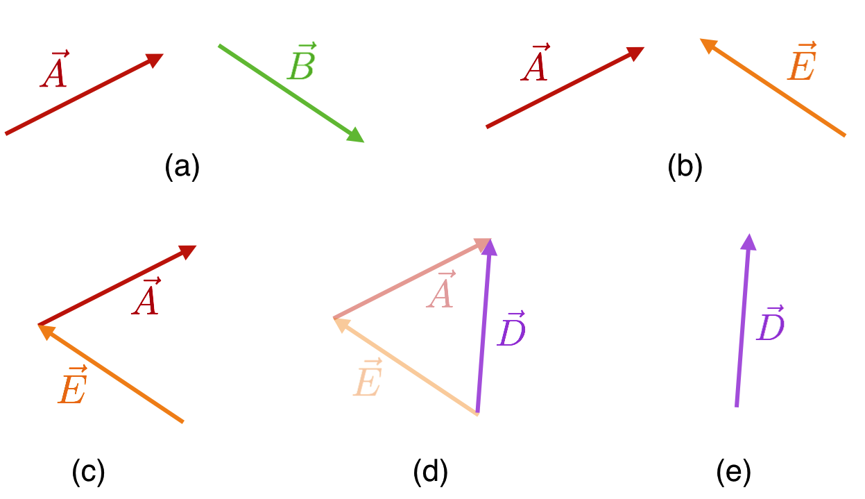
That is everything we’ll need for any vectors that come along in QS&BB!
Approximating Functions
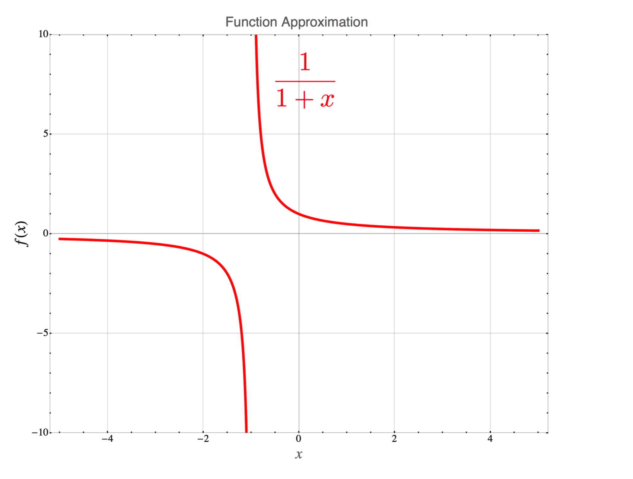
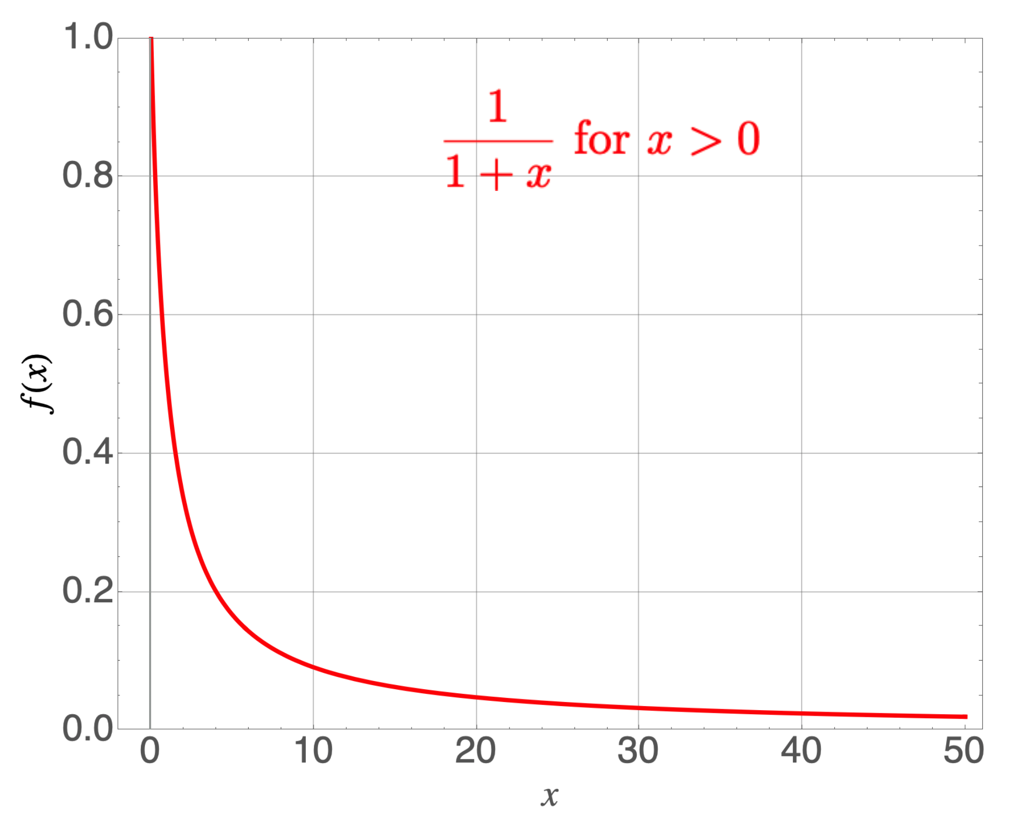
$$y(x) = \frac{a}{b+x}. \nonumber$$ We'll ask this question of a function often:
What is $y$ if $x>>b$
or what is $y$ if $x<<b$?
Here's the thought process you'd go through to answer these questions. For the first one, if $x$ is very much larger than $b$ then that's nearly asking the question, "What is $y$ if $b = 0$?" which is the extreme of noting that if $b$ is really tiny compared to $x$ then it's almost as if $b$ isn't there are all. We'd get:
$$y(x>>b) \approx \frac{a}{x} \nonumber$$ The other extreme would lead you to say to yourself, "If $b$ is huge compared to any $x$, then it's almost as if $x$ isn't there at all." So:
$$y(b>>x) \approx \frac{a}{b} \nonumber$$ This kind of analysis can lead to useful insight to the physics of a particular model. But we almost always want to look at a graph, like here, for the special case in which $a$ and $b$ are both 1:
$$f(x) = \frac{1}{1+x} \nonumber$$
But there’s a more nuanced way of looking at approximations which is due to Isaac Newton. He found a way to represent a function in pieces, for cases in which the power of such a function could be anything: a positive integer, a negative integer, or even a fraction. The pieces add together to perfectly recreate the original function. The bad news is that to do so perfectly requires an infinite number of them! The good news is that one can get very close to the original function with only a few of the pieces. In contrast to how that sounds, it’s actually very useful for many physics applications as we’ll see.
Here’s his expansion for our function:
That last bit of $…$ means that the expansion continues in that pattern for an infinite number of terms.
But notice that each term is a separate function in and of itself. That is, $f(x)$ can be written as the sum and difference of many functions, $1, x, x^2,…$. Add them all up and you’ll get the original function in all of its glory. Add only the first few terms and you’ll get close to the original function. Let’s do that for the first four terms and compare it to the original, full-fledged function.
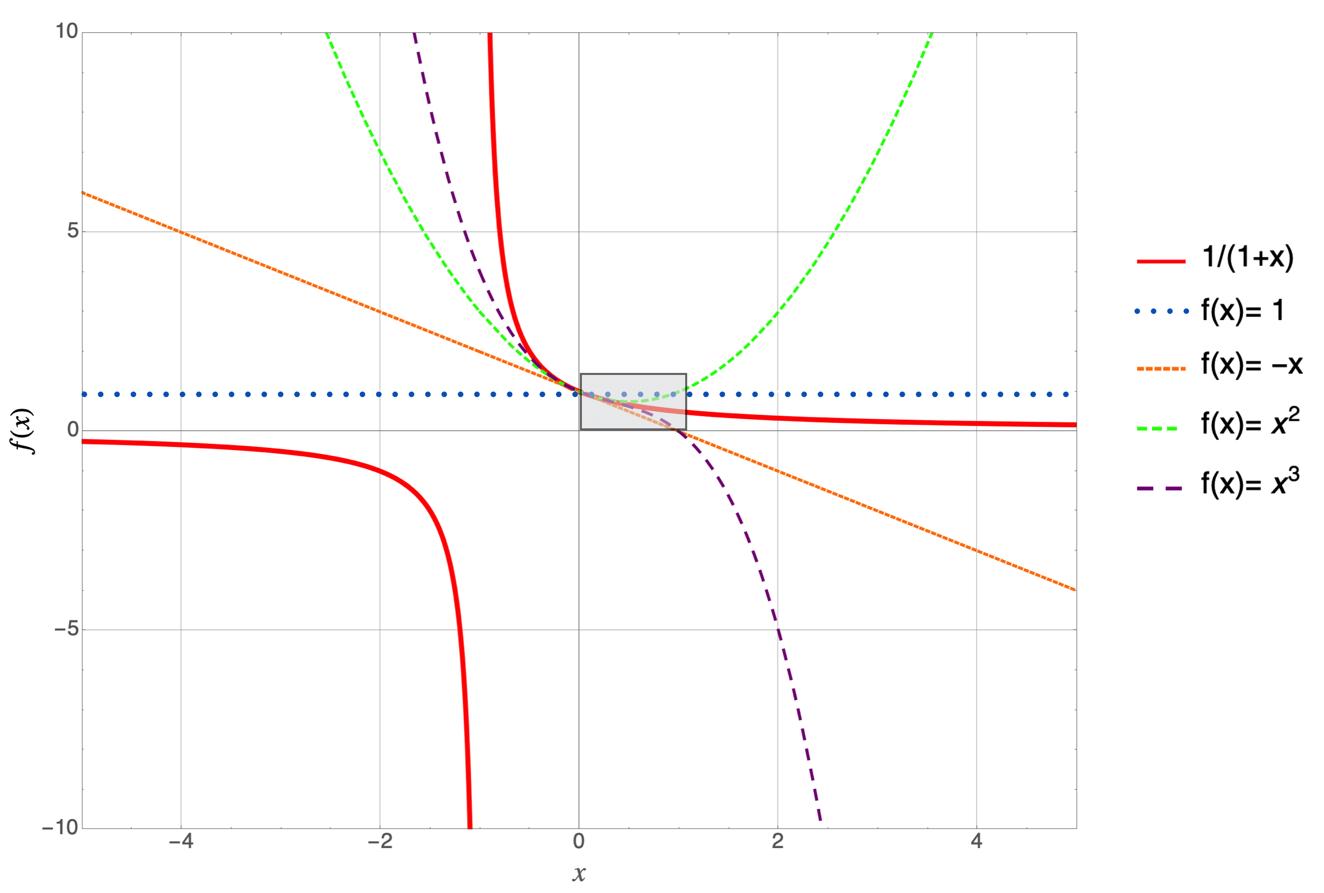 The original function is in solid red and each successive curve adds the next term in the series. So, the blue dotted line is $f(x)=1$, the first term in the series; small dashed orange is adding $-x$, so $f(x)=1-x$; medium dashed green is $f(x)=1-x+x^2$; and finally, long dashed purple is $f(x)=1-x+x^2-x^3$. Let’s zoom into the region in the box.
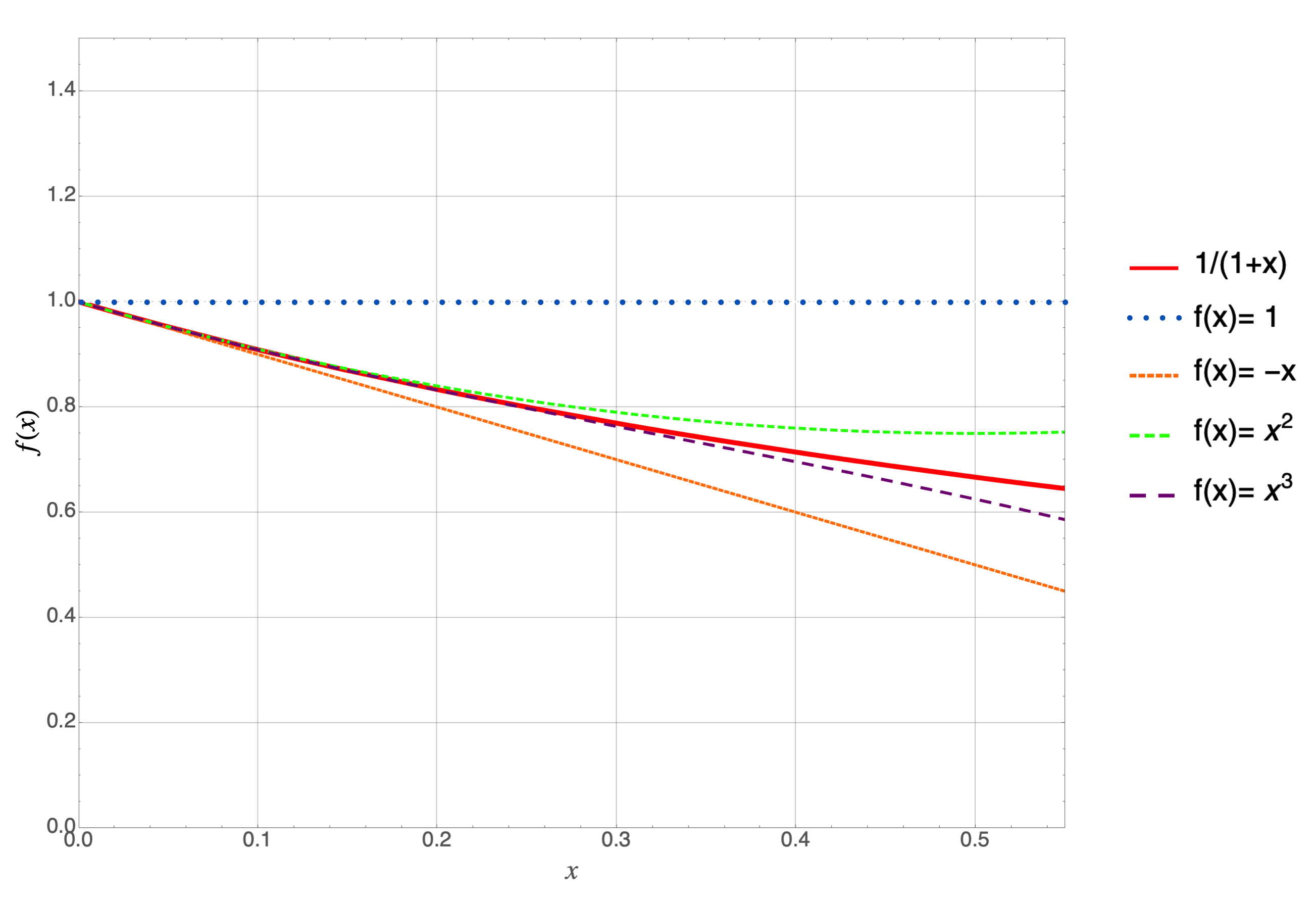 The curves all mean the same thing, except that the $x$ range is now from $0–0.6$ and the $f(x)$ range is from $0–1.5$.
Wait. I’ve had more fun than this…
Glad you asked. Here’s the punchline. You’ll thank me when we get to relativity. Or not.
Suppose that all you cared about was $x$’s that are less than about 0.1 and you need to evaluate the curve quickly, or gain some physics insight for that small of an $x$ region. Then you could get away with approximating
Look at how close the solid red curve is to the short dashed orange curve. Good enough.
Suppose you cared about $x$’s that are less than 0.3…then $1-x$ would not be accurate enough, but the long dashed purple curve would be since it’s indistinguishable from the solid red curve up to that point.
Look how each curve successively makes the approximation better and better as $x$ increases. So if you can be confident that your $x$’s are going to be less than say 0.1, then you can approximate the original function with maybe the first two terms:
since the blue and orange curves when added together are neatly underneath the red curve. The more terms we might add the further out in $x$ that agreement would continue. Add an infinite number of terms—not advisable—and you’d perfectly reproduce the original function.
Remember this! It will become important later when we’ll encounter some physics functions and approximate them with a few terms of the expansions that we’ll encounter. Here are the functions that we’ll see in the lessons ahead:
Thanks, Isaac.
Formulas From Your Past That Might Only Be Referenced Informally
Ellipses and hyperbolas will come up, but descriptively. I’ll just want you to have a feel for their shapes and some of the terms that are defined by them. Just file away this location and we’ll come back only a few times.
Equation of an ellipse
An ellipse is a squashed circle (?) that has two axes, the major axis ($a$) and the minor axis ($b$). The points at which the curve goes through the axes at the major axis points are called the vertices of the ellipse. The equation of an ellipse centered on the origin is
The figure of an ellipse centered on the origin is here:
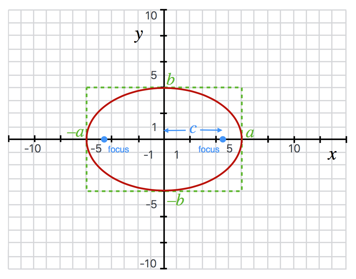 An ellipse with equation $\frac{x^2}{36}+\frac{y^2}{16}=1.$
The focus ($c$ in the diagram) of an ellipse is shown and has the relationship to the curve in that any line connecting one focus to the curve and then to the other focus is always constant. The relationship to the major and minor axes is $c^2 = a^2-b^2.$ So, if $a=b$ then the ellipse is actually a circle and the position of the focus is at the center of the circle, here the origin. The degree to which an ellipse is almost-circle-like (more symmetric) and almost-flattened-like is determined by its “eccentricity,” $e$. It’s defined as $e = \frac{c}{a}$. So an eccentricity of zero is a circle and the larger the eccentricity, the more the focus point is close to the vertex…and the flatter it is.
Equation of a hyperbola
I’ll want to refer to a hyperbola once in QS&BB and it will have a particular shape. This particular form of hyperbola is open to the right and left and crosses the $x$ axis at $\pm a$—the “semi-major axis”—and has a semi-minor axis of $b$ (see the figure). The equation is
The points $(x_0, y_0)$ are where the center of the hyperbola is and in the figure, that’s the origin.
There are a variety of definitions which you can see on the diagram.
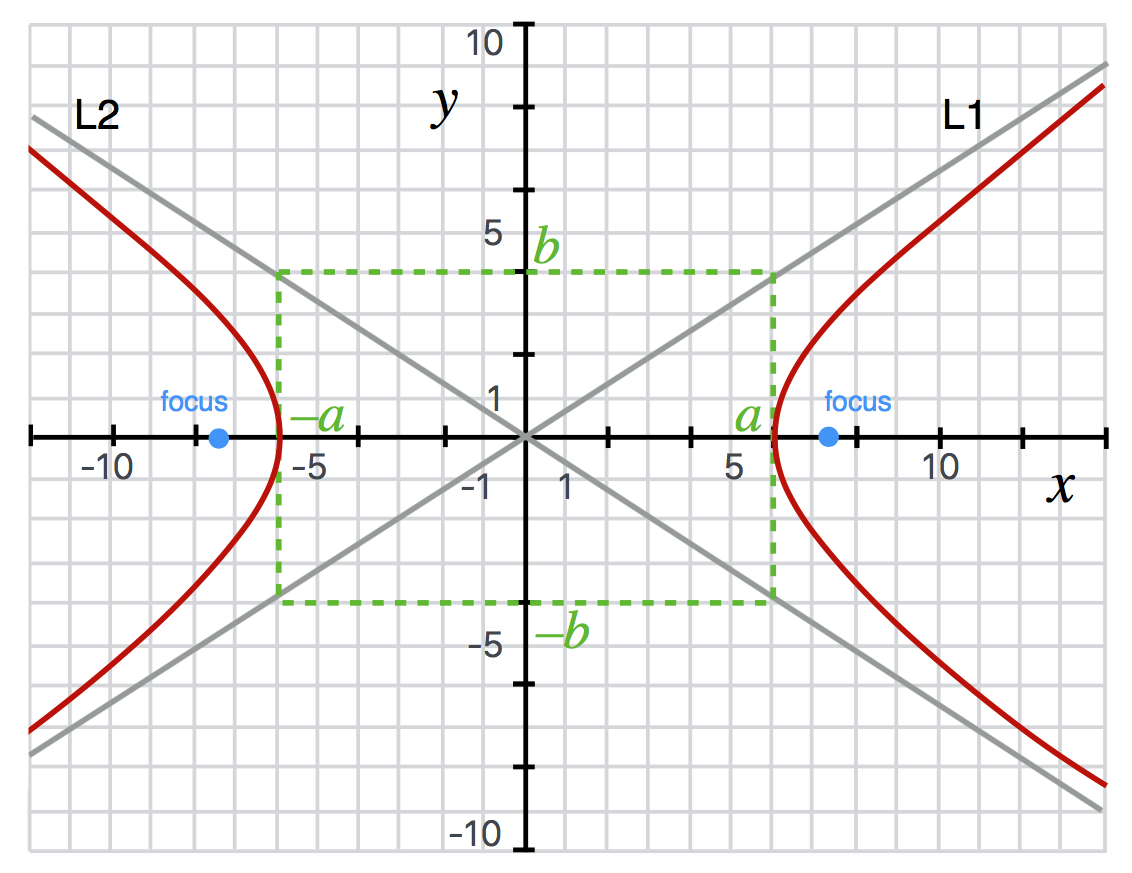 The equation of this hyperbola is $\frac{x^2}{36} - \frac{y^2}{16} = 1.$
What to Remember from Lesson 3?
This has been a whirlwind pass through lots of mathematics from you past. I’d like you to remember that functions are nothing more than little machines for taking a variable and turning it into a value. The world seems to be astonishingly well described by models made up of functions! Some of them are easy and some of them are complex. Only some very simple manipulations will be required. See the Fairness Doctrine of Algebra!
I’ll ask you to “read” functions sometimes, but I promise: only when they are simple and only when there’s physics insight to be gained from that. Otherwise, we’ll be content to read graphs to “evaluate” functions because, well, it’s the same thing.
Powers of 10.
That will be an important tool since we’re talking about the largest things in the universe and also the smallest things in the universe.
Geometry
There are some simple equations, areas, and circumferences of geometrical objects that I’ll need you to remember: line, circle, triangle.
The rest
The rest of the items in Lesson 3 are there for you to refer to when we touch on some science stories that need them.
-
This stands for meter-kilogram-second, as the basic units of length, mass, and time. It’s a dated designation as the real internationally regulated system is now the International System of Units (SI) which stands for Le Système International d’Unités. The French have always been good at this. ↩︎
-
Actually, the Declaration of Independence wasn’t fully signed until August 2, 1776—my birthday! The day, not the year. ↩︎