Contents
- A Little Bit of Huygens
- Collisions
- Impulse and Momentum Conservation and the Third law
- The Simplest Collision of All, Everyday and Quantum Mechanically
- Collision Diagrams: Same Song, Different Verse
- Multiplication by Areas…and Thermometers!
- Two and More Dimensions
- What to Remember from Lesson 6?
Goals of this lesson:
- I’d like you to Understand:
-
The meaning of Momentum Conservation
-
How to use the momentum conservation equation in one dimension
-
How to draw the Feynman Diagram for collisions of two objects
- I’d like you to Appreciate:
- How momentum conservation works graphically in two dimensional collisions
- I’d like you to become Familiar With:
- The history of understanding collisions
- Huygens’ life
A Little Bit of Huygens
Isaac Newton wasn’t the only smart guy around. He had respect for only a couple of contemporaries and Christiaan Huygens, a Dutch gentleman of means—and oh, by the way, a genius astronomer, inventor, and mathematician of such esteem that he was a elected foreign member of the British Royal Society—was one of them. Another was his rival for the invention of calculus, Gottfried Wilhelm von Leibniz. It’s interesting that neither of these two had academic day jobs. Huygens did what he pleased and Leibniz was a diplomat for the House of Hanover for much of his life.
Christiaan Huygens grew up in a privileged household in the Hague where his father, Constantijn Huygens, was a diplomat and an advisor to two princes of Orange. The Huygens’ home was unusual. Guests included Descartes and Rembrandt, whom Constantijn helped support. Constantijn was also a correspondence friend of Galileo, a poet and musician, and was even knighted in both Britain and France. So perhaps it was logical that he would provide for Christiaan’s home-schooling.
When ready, Christiaan was sent to Leiden University to study law two years after Newton was born, whereupon he discovered professional mathematics. A pattern we’ve seen before, although unlike Galileo’s case, Christiaan’s mathematical education had included encouragement from Descartes when he as a child. So his father was much more understanding…and the need for a “job” was never an issue in this family.
Huygens became interested in astronomy and learned to grind and polish lenses in a new way which led to the development of a telescope of unparalleled quality. Among his first discoveries was the large moon of Saturn, named Titan and then the resolution of Saturn’s rings.
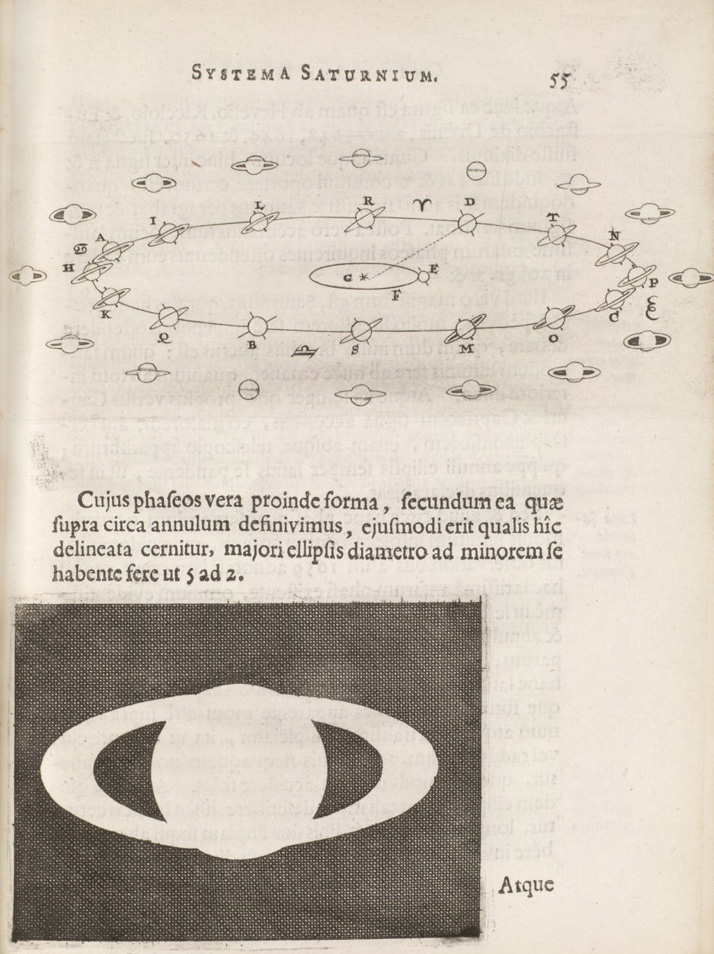
The space probe “Huygens” was designed by the European Space Agency and landed on Titan on January 14, 2005. The arc from Christiaan Huygens’ first glimpse of Titan to the modern photograph of its surface is a nice story.
An increasingly precise program of astronomical observations led him to the need for more accurate time-keeping, whereupon he invented the first pendulum clock (think “Grandfather”)—by fashioning a pivot that made the pendulum swing in the pattern of a cycloid, rather than strictly circular motion of an unhindered pendulum. Galileo had shown that the period of a pendulum was independent of the amplitude of the swing (“isochronous”) but this is only the case when the amplitude is small. Huygens showed mathematically and then by construction that if the bob can be made to take the path of a cycloid, that the motion would be isochronous even for large swings, and hence useful in a clock. He also carefully considered the forces on an object in circular motion and the derivation of the centripetal force in the last lesson was actually obtained first by Huygens for a circle.
However, he was confused by the tendency of an object to move away from the center of a circle and called the force out “centrifugal force.” Newton also was initially confused by this but figured out that gravity, for example would pull in and hence coined the name “centripetal” to contrast it to Huygen’s idea. Newton’s analysis was general and included circular, elliptical, parabolic, and hyperbolic orbits, so we tend to credit him with the correct understanding of curved motion.
Huygens traveled widely and spent considerable time in Paris in multiple long stays. He visited Britain many times as well, and when he thought he was dying (he was often in frail health) he bequeathed his notes to the British Royal Society. (He recovered.) His scientific circles were very broad and he counted as among his friends most of the intellectuals of the day, including Boyle, Hooke, Pascal, and indeed, Newton whom he visited shortly after Principia was published. Christiaan Huygens died at the age of 66 four years after his visit with Isaac Newton, who referred to him as one of the three “great geometers of our time.”
For our current purposes, it was Huygens’ consideration of collisions that is his legacy. Descartes had considered the problem of colliding two objects together and he applied his notion that all motion in the universe is conserved to such problems. But he was confused about just what was conserved and didn’t have an appreciation of vectors or momentum. Putting Huygens’ work together with Newton’s gives us our modern ideas about how the total momentum of a system of colliding objects is preserved and that’s our concern in this lesson.
In particle physics we’re all about collisions and we construct huge, international facilities to do nothing but crash things together. Yet we still use the same ideas and language first invented in the 17th and 18th centuries, albeit fancied up for modern applications.
Collisions
One of the treasured concepts for physicists is the idea of the conservation of some quantity. We’ll make use of that idea over and over.
While we have a sophisticated justification for this affection for conserved things, even before Conservation Laws were a notion at all, natural scientists had an intuitive sense that nature seemed to preserve some qualities. The first such serious assertion became known as the “Conservation of Momentum.” Descartes started it all when he declared that the total “amount of motion” is unchanged, just shared among all of the various bodies in the cosmos.
His model of the universe assumed that it was originally kick-started with all of the material bits set into initial motion and all of this primordial motion shared among all objects forever—a little given up over here means that it shows up over there. The total is preserved, or “conserved.” Add those individual bits of motion up at any time and you get the amount of motion you started with. “Bits of motion” for him meant: speed.
This eventually led him to his Big Idea that outer space was (had to be?) filled with various sized balls which were originally rotating together in a great “vortex,” and in that way dragging and pushing the planets along with them. Think of a ball pit for kids (fun, but a veritable petri dish of bacteria.) Those balls constituted his choice as material cause of the orbits of the planets.
Wait. What balls?
Glad you asked. You mean how did he come up with this idea? As a materialist he felt that he was forced to invent a cause: some contact force between objects to make anything move, including the planets. Descartes’ philosophy influenced his science: it was top-down. Postulate a cause and then work it out. But don’t ever postulate a kind of motion without first setting up the mechanism that creates it. His commitment meant: I see the planets moving, so something has to be pushing them. Material, but invisible balls sharing the original primordial motion is as good as anything else.
Newton dismantled Descartes’ vortices but after considerable massaging the preservation of the total motion was an idea that was still around after Newton was finished. Certainly, we now attribute planetary motion about the Sun as reflecting the original rotation of the random space-dust that nearly five billion years ago slowly coalesced into their solid masses. Still orbiting, after all these years.
Everyday Collisions
Let’s look at some collisions that we all could create using everyday objects. I’m aiming toward a symbolic and pictorial approach with only minimal mathematics.
Wait. Apples?
Glad you asked. Well, we could collide apples but that would be messy. When we get to quantum mechanics and particle physics you, like I do, will probably have “billiard balls” in your head. Let’s just think do that…head on.
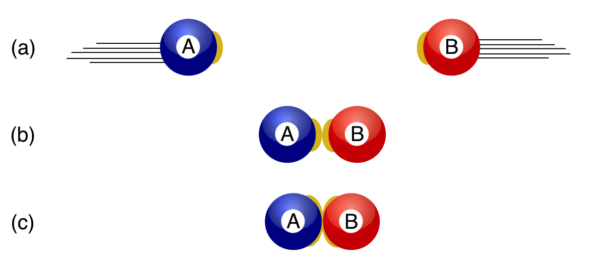
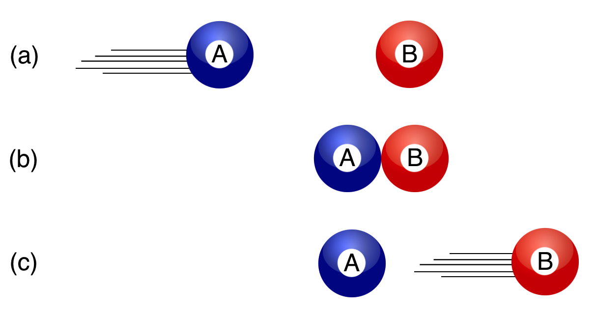
Here’s a very familiar collision in three scenes from the top, to the bottom: (a) before, (b) during, and (c) after the collision of two identical, rigid, frictionless balls. Yes, billiard balls is one of ways that we’ll abstract from real-life collisions to ideal ones. Here you go:
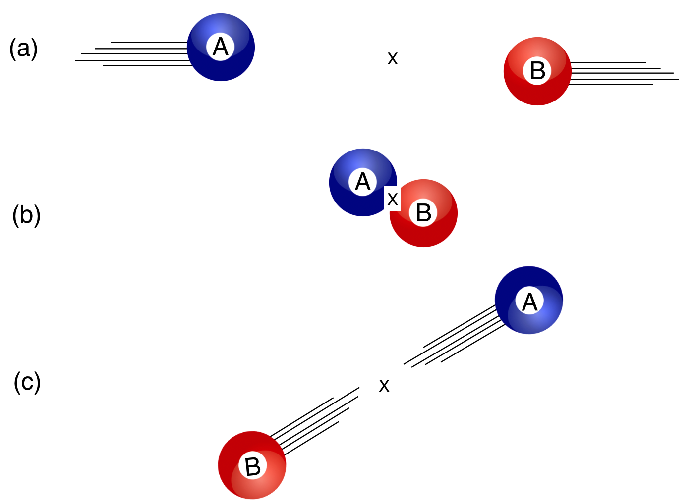 Two identical billiard balls are moving towards one another with the same speeds in (a), collide at (b), and recoil from one another at © Notice that they’re slightly off-center which is necessary in order to get them to recoil at an angle.
- First, in order for these two balls to change their motions from totally horizontal [(a): before], to obliquely scattering to directions with both horizontal and vertical momenta [(c): after], they need to collide off-center [(b): during]. So obviously, these particular billiard balls have a size. When we deal in quantum particle collisions, the sizes are so tiny that it simply works to treat them as point-like: no size at all.
- Second, by setting up the situation with no friction, we’ve left the realm of real billiard balls which roll. Rolling is entirely due to friction (think of your car’s tires on ice). Our colliding objects could be in outer space, barreling along without friction.
- That they are “rigid” means that when they collide their material does not compress at all. In real materials, there would be some “give” that would vibrate and dissipate as heat in the ball and vibrate the air producing sound. Our ideal collisions are called “elastic,” which we’ll explore in the next lesson.
- Finally, no two things in our everyday life are absolutely identical. If you’ve studied any philosophy, you might recognize some of Plato’s reasoning. Real billiard balls would be copies of the Ideal Billiard Ball for him. We nod to Plato but we allow absolutely identical objects in our working-ideal world. (But in the quantum world, all like-objects are absolutely identical—every electron is like every other electron—and that will become an interesting chapter in our QS&BB quantum mechanical story!)
Wait. There you go again. You’ve decided to describe an unrealistic circumstance. How is that helpful?
Glad you asked. Remember, when we build a model we do it in a way that emphasizes the dominant physics at the expense of any less significant, but realistic effects, that would get in the way of a simple description. In this case it’s also a pretty good approximation for many real situations. Likewise if we shot one electron toward another election their electrostatic repulsion is responsible for the recoil and it’s almost perfect. So this is a pretty good model for us.
By the way: our concern in particle physics is the [(b): during] part of this interaction. That’s where the guts of the physics lives and nature’s rules are at work.
Wait. Sorry to bother you again so quickly. Isn’t the “during” here just that the two balls touch and recoil?
Glad you asked. No problem. That’s the neat thing about, well, everything. There isn’t a rule or a force of nature called “touching.” The rule of nature at work here is the same one that keeps you from falling through the floor: the electromagnetic repulsion of the electrons near the surface of each of the balls is the actual force at work in “during.” One of only four known forces. But stay tuned.
This ideal two dimensional collision is mathematically more complicated than we’ll need. I wanted to start with something familiar. Let’s categorize our collisions by writing little reactions and drawing diagrams to describe them.
Everyday, But Ideal Collisions
You have all collided one thing with another, whether in a game (on purpose) or your car (not on purpose!)—one thing banging with another thing is a well-known, and sometimes personal event. I’ll refer to collisions many times and in this section we’ll collect a set of representative kinds of collisions for future reference.
Collision 1: $\mathbf{A}+\mathbf{B}\to \mathbf{A}+\mathbf{B}$
Let’s start simply with two billiard balls which are in a head-on collision, that is, not off-center. For this first collision, the objects are identical but they’re labeled separately as $A$ and $B$ in order to keep track of them. At the LHC, they would be identical protons. In billiards they would be different colored balls. We can describe these or any collisions of two equal particles in, two equal particles out, with the same “reaction” formula: $\mathbf{A}+\mathbf{B}\to \mathbf{A}+\mathbf{B}$ (or maybe you’d prefer $\mathbf{A}+\mathbf{A}\to \mathbf{A}+\mathbf{A}$?).
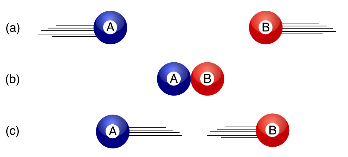
In Collision 1 the two balls retain their identities after they collide: you (a) start with an $A$ and $B$ at the beginning and you (c) end up with those same pair of $A$ and $B$ at the end, none the worse for wear. In (b) they collide and if they’re everyday objects, you could take a picture and see them touch.
I’ll bet you know what would happen if they are identical in mass and their initial speeds, $v$, are the same. Descartes would have said that the total speed at before they collide is $2v$ and so the total speed after they collide would also be $2v$. And he would be sort of right—but for the wrong reason (most of us hate it when that happens). In this collision, both balls would recoil from one another and just reverse their original motions.
But this a special case since one could be faster than the other in (a) or one could even be sitting still: at rest. Then their final speeds will be different and Mr Newton and Mr Huygens wrote down the rules that enable us to predict the results: you give me their states at the beginning (remember, a state means knowing positions and momenta) and I can tell you their states at the end. The middle is where the physics action is since a collision like this could be two actual electrons which would repel one another without ever touching. Stay tuned.
Collision 2: $\mathbf{a}+\mathbf{B}\to \mathbf{a}+\mathbf{B}$
A variation on Collision 1 is when the two participants have different masses or different natures altogether. The reaction formula looks similar, but I’ll call out the lighter one with obvious notation: $\mathbf{a}+\mathbf{B}\to \mathbf{a}+\mathbf{B}$.
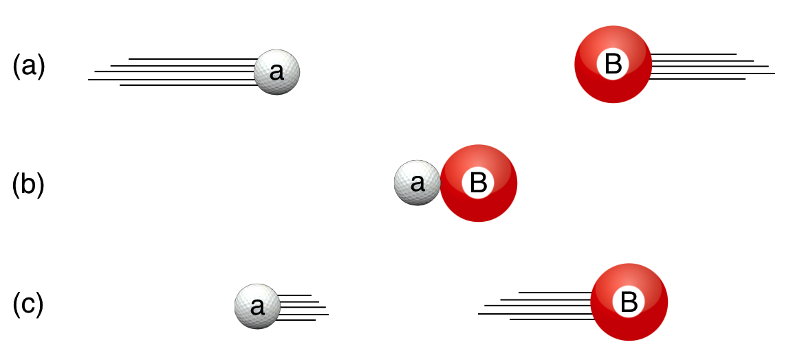
Think a 180 lb safety, stiff-armed and bouncing off a 250 lb running back. Those collisions are not symmetric and are heavily dependent on the initial speeds and masses. Collision 1 is really a special case of Collision 2, which is the most general everyday (ideal) collision between two, different objects.
Collision 3: $\mathbf{A}+\mathbf{B}\to \mathbf{C}$
If two of you are really good, you could add glue to a couple of billiard balls and precisely throw them at one another with exactly the same speeds. They would stick and stop dead, becoming one object (C) made up of the original two. (We’ll see why in a moment.)
Wait. That doesn’t sound like a good idea.
Glad you asked. I agree. But these are ideal collisions, so let’s pretend that you two are ideal throwers.
Here’s the picture (see the glue?):
Here, Descartes got it wrong: he would have said that the original motion was $2v$, but we know that the final “motion” is $0$.
Obviously he didn’t appreciate the importance of the directions of the velocities in the addition to their magnitudes. That is, he didn’t know about vectors. In the sticking-together collision we instinctively know that the result is: $v_A-v_B = 0$ so that they stop.
Speed Is Not the Thing: Momentum is the Thing
Speed is not the conserved quantity. Rather, Newton’s momentum was the key, defined as the vector quantity, $\vec{p} = m\vec{v}$, with both a magnitude and direction. He had the beginnings of an appreciation for the direction of momentum, filling a concept-gap that neither Descartes nor Galileo had come to on their own.
Huygens got it right: he understood the idea of vectors, although in an entirely different and complicated way that got sorted out by the 19th century into the language that we use today.
Collisions were a fascinating study for those working in the 17th century. Everyone understood that friction confused the real picture, so people relied on colliding pendulums where these effects were reduced. One has visions of everyone having many “executive toy” contraptions in their workrooms, changing out the bobs and causing clacking collisions with careful measurements of the outcomes. Huygens made use of his home-town canals in Amsterdam as way to collide masses in a controlled way. Amsterdam’s canals provided a near-frictionless racetrack for accelerating particles. He would station a colleague on a canal-boat with a pendulum which would collide with one held by someone on the shore. As the boat went by, nearly frictionless collisions were created and, he was able to get study the collision from the point of view of a “fixed” coordinate system (say, the shore-guy when the boat-guy went by) and the “moving” coordinate system (the boat-guy). His geometrical explanation was very complicated, but essentially correct. I’ll describe it here in modern language.
Back to Collision 3 with the glue: if $A$ and $B$ are different masses, but they still stick, they would still make a third object (C). The idea is the same: two objects become one object. That’s the situation of our safety and running back where the safety hangs on and really tackles the runner. Or, where a baseball is caught by a fielder, again, two objects becoming one. Together, they’re a third object.
Collisions 1-3 are all of the collisions that can happen in one dimension with two everyday objects. But this is QS&BB, so there’s more!
Quantum-like Collisions
Let me show what kind of strange things can happen in quantum mechanics, with a little artistic license using everyday objects as stand-in for quantum particles.
Collision 3, again: $ \mathbf{A}+\mathbf{B}\to \mathbf{C}$
Weird Happens in quantum mechanics. We know how to prepare initial quantum states, (a). Our particle beams do that for us. We know how to detect what comes out of a collision, (c). The detectors we build do that for us. It’s what happens at (b) when the collision actually happens that’s interesting and because quantum mechanics—and relativity—are involved.
Here’s a quantum mechanical version of the glued-billiard balls:
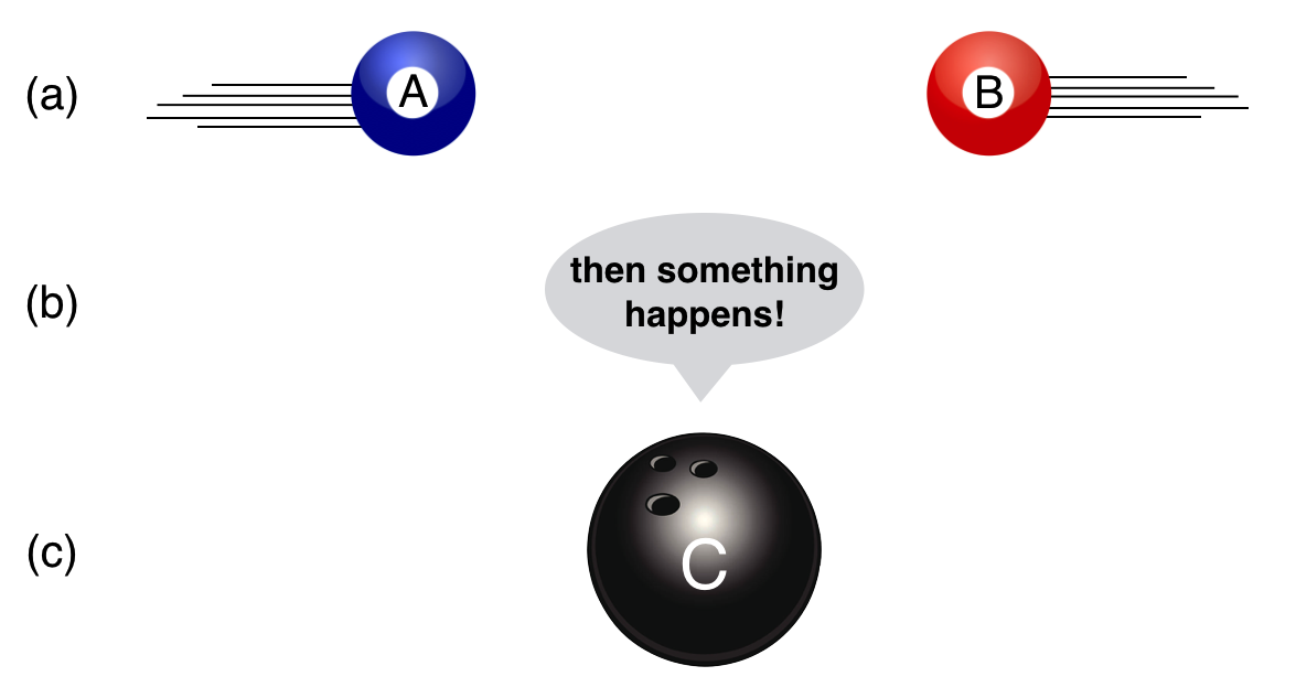
A little different in two ways. First, what comes out is not a recognizable combination of $A$ and $B$, but something else entirely. Second of all, what happens at (b) is now the question:
Modeling how quantum particles interact when they’re near one another is one of the goals of particle physics.
Collision 4: $\mathbf{C} \to \mathbf{a} + \mathbf{B}$
A more common situation is sort of the opposite of Collision 3:
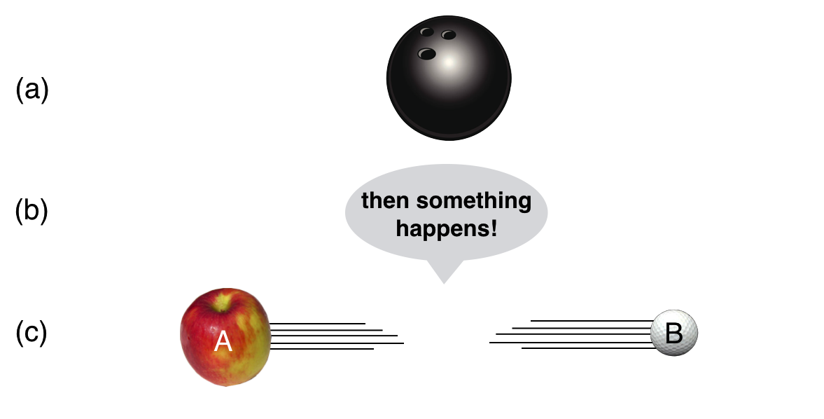
Here we’ve got a quantum particle sitting there minding its own business (the bowling ball) when suddenly it disappears and two (or more) entirely different quantum particles are created…seemingly out of nothing. This was quite the shock when “decays” like this were observed in the 1890’s and we’ll talk about some of these discoveries. Now we know how to describe this process but surprising decays are often the signature of brand new kinds of physics. A firecracker going off is the closest we to a quantum decay that have in everyday life. But firecrackers don’t explode on their own and the results are not only two or a few objects.
Collision 5: $\mathbf{a}+\mathbf{B}\to \mathbf{c}+\mathbf{D}$
Collision 5 is a standard quantum collision of two initial quantum particles which collide—doing something in the intermediate (b) state—and then completely transforming into two or more entirely different objects, (c).
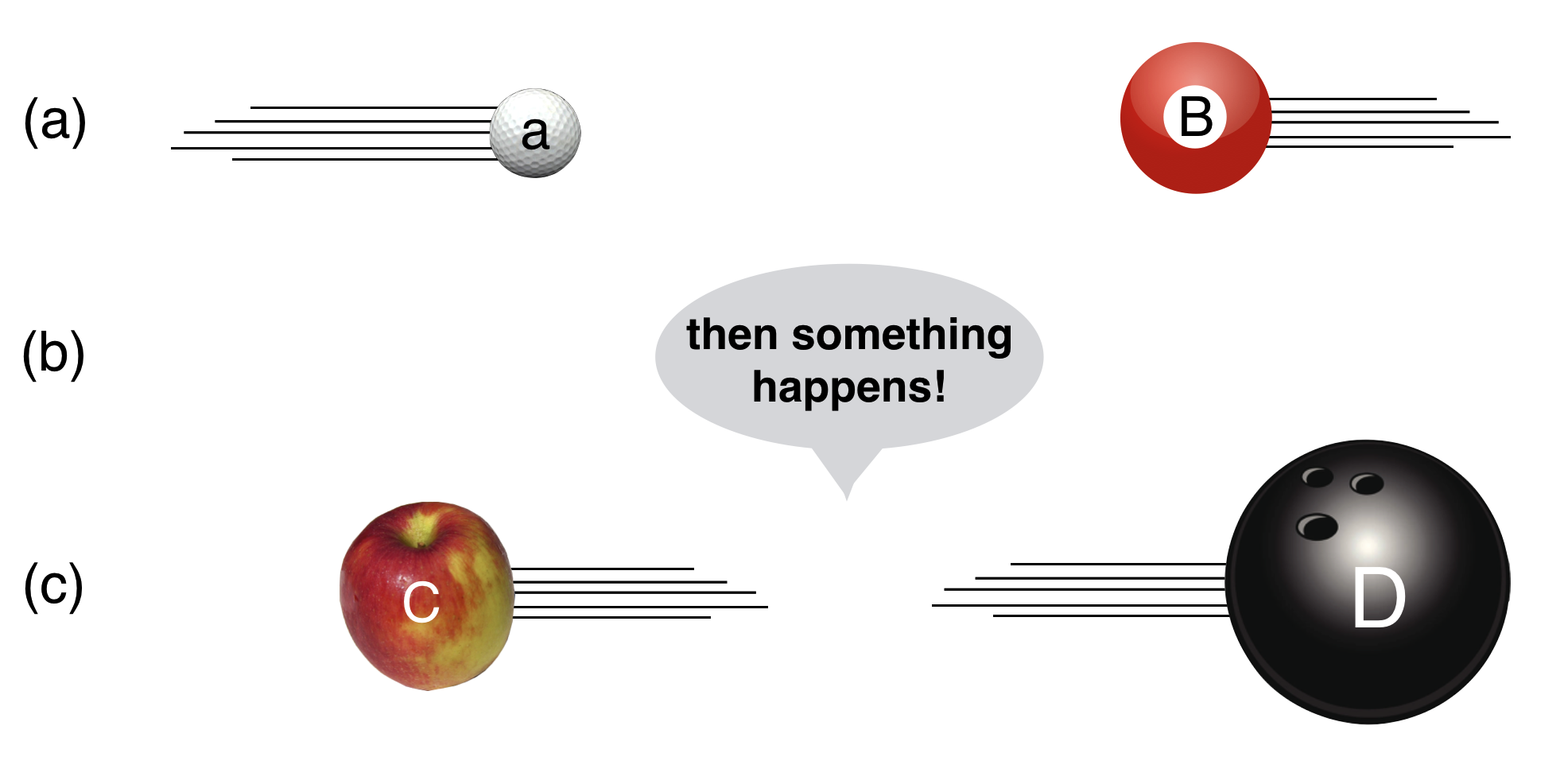
There is no everyday analogy for this. It’s as if our safety and running backs collide and become a baseball pitcher and an Oldsmobile. Creating an obsolete GM car would be a surprise indeed, but that’s how we discover new particles and study unusual forces of nature.
Quantum collisions can take ordinary matter and produce entirely different states of matter.
🖥️ Please answer a question:
🖥️ Please answer a question:
🖥️ Please answer a question:
Impulse and Momentum Conservation and the Third law
A conserved quantity in physics is one that is unchanged during a time interval—typically a “before” and “after” some event. These statements are called “ConservationLaws.”
Let’s work out the most important one of these and get to know it. It’s inventor? Why, Mr Newton, which should be a surprise to no one.
You can make two simple, but important observations from this:
When they just start to make contact your left hand begins to exert a force on your right hand and your right hand exerts a force on your left. Is there any difference? Does one hand fly away from the other? No...from Newton's 3rd law, these forces are equal (and opposite). So let’s name your hands. Feel free to write on your palms: $$\begin{align*} F_\text{left} &= F_A \\ F_\text{right} &= F_B\end{align*}$$ We’re recreating Collision 3 (but without glue). They have opposite directions, so while the magnitude of the forces is the same, the directions are opposite: $$F_\text{A} = - F_\text{B}. \nonumber$$ Is the time that your left hand is in contact with your right hand any different from the time that your right hand is in contact with your left? No, of course not. So: $$\Delta t_A = \Delta t_B \nonumber$$ So let's put these two silly (but not silly!) observations to work. Look at the impulse experienced by any two colliding objects A and B (your two hands). Here are those relations that describe their changes in momentum: $$\vec{F}_A\Delta t_A = \Delta \vec{p}_A \nonumber$$ $$\vec{F}_B\Delta t_B = \Delta \vec{p}_B \nonumber$$ And as we learned "by hand," (see what I did there?) both, $F_A = -F_B$ and $\Delta t_A = \Delta t_B$. So: $$\begin{align*} F_A\Delta t_A &= - F_B \Delta t_B \text{ …giving us:}\\ \Delta p_A &= - \Delta p_A\end{align*}$$ Let's pretend that their collision is in one dimension and remember the convention for “change of” and that we'll use the subscript “$0$” to indicate the initial quantities: $$\begin{align*} \Delta p_{A} &= p_{A} - p_{A,0} \nonumber \\ \Delta p_{B} &= p_{B} -p_{B,0} \nonumber \end{align*}$$ Putting them together, we then find: $$\begin{align}\Delta p_{A} &= - \Delta p_{B} \nonumber\\ p_{A} - p_{A,0} &= - (p_{B} - p_{B,0}) \nonumber\\ \text{rearrange} &\text{ these terms...} \nonumber \\ p_{A,0} + p_{B,0} &= p_{A} + p_{B} \label{pcon} \end{align}$$
Take a deep breath and remember where you were at this moment. Seriously.
Eq.\eqref{pcon} is a really important relationship. First, it’s the statement of “momentum conservation.” Second, it is what’s behind the otherwise, bumper-stickery, out-of-the-blue-sounding “For every action there’s an equal and opposite reaction.” Newton’s third law? Just a memorable and wordy way to state momentum conservation…where the rubber really meets the road, so to speak.
Here’s one of the apparently true things about the universe:
Momentum is always conserved.
…drops mic…which bounces, according to momentum conservation.
The Simplest Collision of All, Everyday and Quantum Mechanically
Now let’s put it to work by solving the simplest collision of all.
Before tackling it, let’s also establish some terminology, some of which is repurposing everyday words into specialized physics terms:
- I’ll use the words collision and scatter interchangeably.
- We’ll often call the whole scattering process—objects approaching, colliding, and separating—an event.
- The state of an object is its particular values of position and momentum. These six quantities are enough to completely characterize an object’s future motion.
- Let’s treat the moment of collision as a special time in the event serving to separate the initial state [before, our (a)] from the final state [after, our (c)]. So an event consists of the initial state, the collision, and the final state.
- For our purposes, we’ll reserve the phrase elastic collision to mean that the two objects that scatter at the beginning are the same two objects after they collide. They have different states, but they are still the same objects in an elastic collision.
- We’ve already met a decay which is an atomic, nuclear, or particle physics idea.
- And, a reminder about units: remember that the units of momentum are associated with the units of $p=mv$ , so mass times velocity. So a kilogram-meter-per-second is a perfectly good unit for a momentum. In the English system, so would be slug-ft-per-second, which is a lot of fun to say, but it’s not usually used.
But these units are unfamiliar and could get in the way of grasping the important stuff, so let’s just invent our own unit-less arbitrary measure. If I say that a particular momentum is “5,” we’ll interpret that to be in arbitrary, fake “momentumunits.”
Two more terms which repurpose some regular words:
- Beam. Any of our objects that are moving toward a collision, we’ll call a beam or beam particle.
- Target. A beam is aimed at an object which we’ll call it a “target.” Just what is the target and what is the beam is a matter of your point of view, but it will be clear in our contexts. You’ll see.
The simplest collision of all is when the target is sitting still and the beam hits it—like our billiards or ice hockey example. This situation is called a Fixed Target Collision.
Let’s play pool.
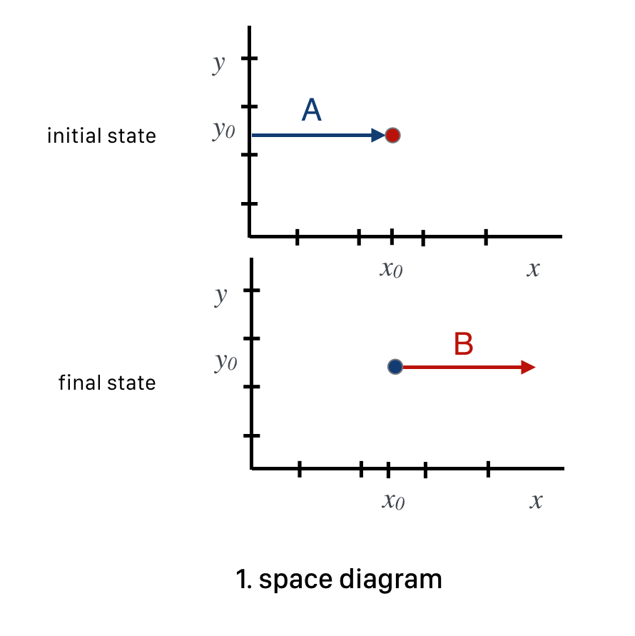
The Stop-Shot, Elastic Scattering With a Wrinkle: $\mathbf{A}+\mathbf{B}\to \mathbf{A}+\mathbf{B}$
Here is the simplest collision of all. It’s a variant of Collision 1 when the $B$ ball is sitting still minding its own business and cruelly struck by $A$. Here it is:
You’ve done it with billiard balls: the first one comes in, strikes the stationary one, and it scoots out and the first one stops in its tracks. Can’t get any simpler. It’s called a “stop shot” or “dead ball shot” in pool and here it is in a clip:
Here, Momentum Conservation will be on trial. Let’s go step by step through this long example.
Wait. Do I have to?
Glad you asked. Well, no. Of course you don’t “have to” but if you just follow the path, you’ll end up knowing a lot more than you do now!. Please do it?
In our fake “momentumunits” let’s invent an example and follow it through. If you can do this kind of thing, then you’re in good shape to understand any scattering process.
An Example: The Stop Shot
- We’ll make the initial momentum of the cue ball to be “12,” in our fake units: $p_0(A)=12$
- B is initially sitting still, so the initial speed of the B is zero, $v_0(B)=0$.
- The mass of each ball is 6, so $m(A)=m(B)=6.$
questions
- What is the initial momentum of the B ball?
- What is the initial speed of A?
- What is the total momentum of the entire initial state?
- Using your experience and the video, what is the final momentum of A, $p(A)$?
- What’s the total momentum of the entire final state?
- From our observation and momentum conservation, what is the final momentum of B, $p(B)$?
- From our observation and momentum conservation, what is the final speed of B, $v(B)$?
Before looking at momentum conservation, we can deal with the first three questions easily:
Answer 1. If the B ball is stationary, then its velocity is 0 and so its momentum is 0, $p_0(B)=0$.
Answer 2. If the intial momentum of A is 12, then the speed of A we can get easily from the definition,
Answer 3. The total momentum of the “entire intial state” is just the sum of all of the individual momenta of all of the objects in the initial state. Let’s call that $P_0$ without any A or B label. In this case,
Answer 4. Our experience is that in the final state the beam ball stops, so $p(A)=0$.
Answer 5. If we name the total momentum of the entire final state to be $P$, in solidarity with the entire initial state momentum of $P_0$, momentum conservation says that
so that if $P_0=12$ then $P=12$ as well.
The final two questions require that we make use of momentum conservation. Let’s set up a table (which you might do in your head some day) and you can think of balancing things. Remember, conserving momentum here means enforcing:
Here’s the table in which we need to supply the missing $a, b, \text{ and } c$ in the right hand column:
Before (initial state) After (final state) total $P_0=12$ $P=c$ A $p_0(A)=12$ $p(A)=a$ B $p_0(B)=0$ $p(B)=b$ sum to: $12+0=12$ $a+b$
In the Before column we’ve listed what we knew. We need to fill in the After column. Let’s take them one at a time:
- What is $c$? The first line is easy since we’ve already done it in Answer 5: momentum conservation insures that c has got to be the same as the initial state’s total, so $c = 12$.
- What is $a$? Our experience tells us that when we strike B with the A that the A suddenly stops dead (Answer 4.) and B jumps forward. So our experience and the video would tell us to put in zero for the final momentum of A, so $a = 0$.
- What is $b=$? Of course it’s 12 from momentum conservation and that’s the answer to question #4.
The last question, 7, asks about the speed of B after the scattering event. Since the mass is 6, $m_B = 6$ and the momentum is $p(\text{B})=12$, then we can see easily that $v(\text{B})=12/6 = 2$ and B goes scooting away with the same speed as A had before the collision.
So this next table completes our understanding of this collision, using experience as our guide.
Before (initial state) After (final state) total $P_0=12$ $P=c$ A $p_0(A)=(6)(2)=12$ $p(A)=0$ B $p_0(B)=0$ $p(B)=(6)(2)$ sum to: $12$ $0+12=12$
Houston, we have a problem
We used our experience to determine the final state. But that’s cheating. We should be able to fully predict the outcome. Let’s try that, but first buckle your seatbelt.
Of course, we know that $B$ is stationary, $v_0(B)=0$. So, we get: $$\begin{align} v_0(A) &= v(A) + v(B). \label{scattersimple} \\ v(B) &= v_0(A) - v(A) \nonumber \end{align}$$ Equation \eqref{scattersimple} is Descartes’ idea again: the total “motion” of the first object at the beginning is not lost but shared between the motions of all of the objects after the collision.
But we’re not happy. No, not happy at all.
Equation \eqref{scattersimple} is a simple, but terrible result! The beam object should stop dead. We just saw it with our own eyes. If our model is complete, then it should predict that: $$v(B) = v_0(A) \nonumber $$ but it's not! It's $v(B) = v_0(A) - v(A)$ which includes the correct result, but isn't uniquely that result.
Wait. You mean that Newton and Huygens were wrong?
Glad you asked. I tried to be careful above in with my, “If our model is complete.” We need more physics! A subject for the next lesson.
Collision Diagrams: Same Song, Different Verse
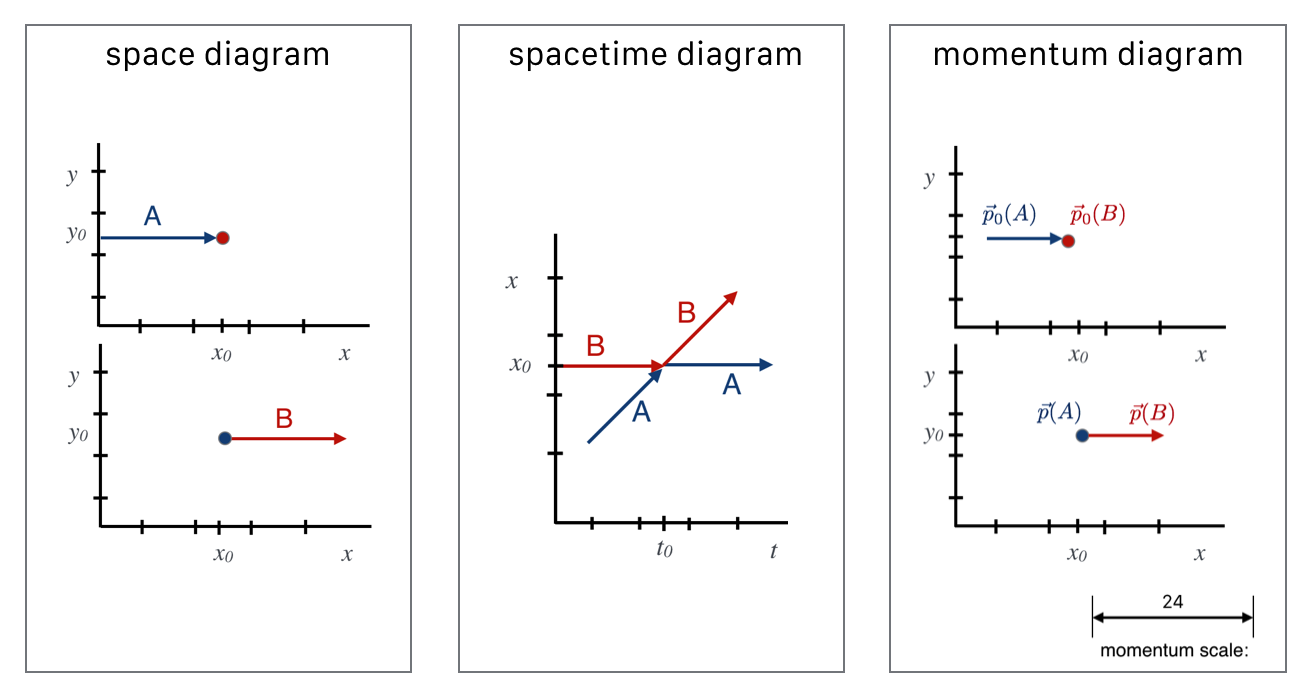
I want us to become familiar with three kinds of diagrams for collisions: space diagrams, spacetime diagrams, and momentum diagrams.
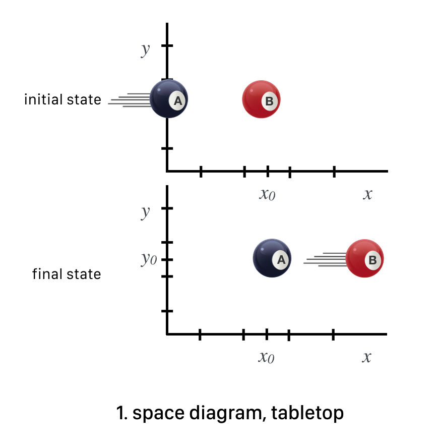
Space Diagram
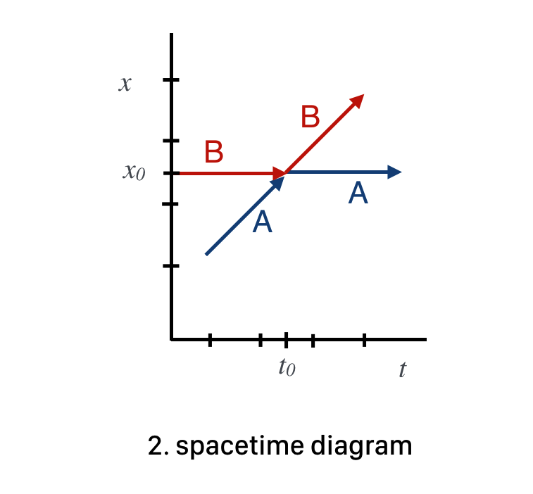
Spacetime Diagram
Momentum Diagram
It’s also useful to include another diagram…one that represents the collision in a “mathematical space” that’s sort of overlayed on the regular $x-y$ space but is vectors of momentum, not displacement. Since a momentum vector points in the space $(x,y,z)$ direction of the velocity, we can do this. But now the length of a momentum vector will be the value of the mass times the velocity. This figure is a collection of momentum vectors using our fake units.
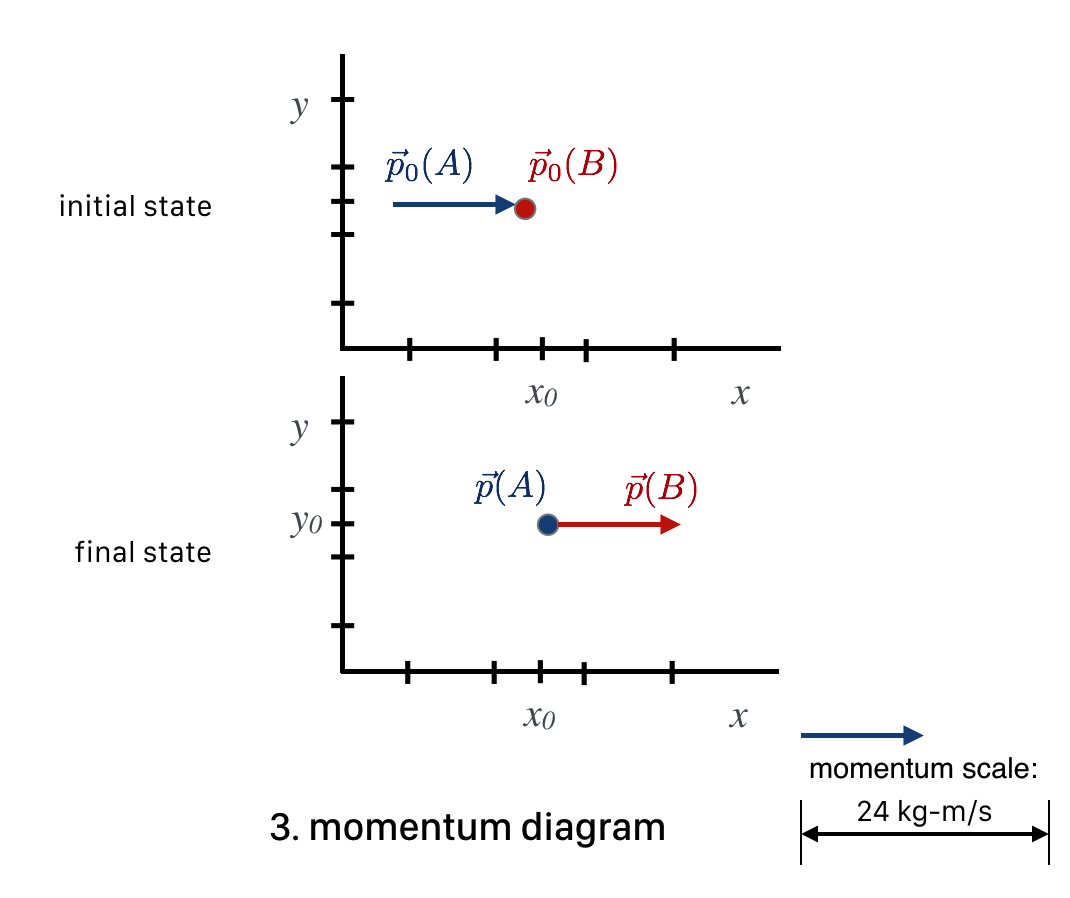
Look at this. Momentum $p_0(A)$ is the original "12" momentum of the $A$ ball and the dot signifies the initial $B$ momentum as a vector of zero length—no velocity or momentum at all. Likewise, the final state has the situation reversed. Notice that the sum of the momentum vectors in the initial state—the total lengths of the vectors (12 and 0) is equal to the total length of the momentum vectors in the final state. Momentum conservation is expressed as a geometrical relationship among the initial and final state vectors.
Let’s summarize all three diagrams here:
📺
Go to 6.6_diagrams_v3_w2m for review and wrap-up of these sections.
Multiplication by Areas…and Thermometers!
When you use equations for a living, after a while they take on visual properties that you learn to rely on. They speak to me like a second language might to you. But when you don’t use equations for a living, I still think that the same kind of physical insight can be gained by continuing to construct geometric diagrams that do the job solving the equations of physical models. This is really useful when we begin to consider conservation of momentum and other conserved quantities that we’ll discover. Let’s quickly look at the stop shot using areas and then we’ll “graduate” to a more straightforward approach: “thermometers.”
Momentum as areas
In our stop shot example, A colliding with the resting B and then B jumping forward leaving A stationary. We were given the following information:
🖋
- The mass of each ball is 6, so $m(A)=m(B)=6.$
- The speed of the cue ball was $v_0(A)=2$.
- So the momentum of the cue ball was $p_0(A)=12$
- $B$ was initially sitting still, so the initial speed of the $B$ was zero, $v_0(B)=0$.
- Therefore, the initial momentum of $p_0(B)=0$
Then we found:
- The final speed of A was $v(A)=0$
- So the final momentum of A was $p(A)=0$
- The final momentum of B was $p(B)=12$
- And so the final speed of B was $v(B)=6$
We can describe momentum and keep track of the directions, if you’ll allow me to define a “negative area.”
Wait. Negative area? What universe are you working in?
Glad you asked. Well, you’ll see what I mean and why I give it such a silly name. (Shhh Don’t tell anyone.)
Let’s set up our area space. We’ll put mass on the vertical axis and velocity on the horizontal axis, but we’ll keep track of the sign of the direction of the velocity by first, defining a particular direction to be positive and second, by then putting our area in the positive ($>0$) $v$ direction or the negative $v$ direction according to the circumstances.
We’ll then define the direction of the cue ball, let’s call it “North,” as our positive $x$ direction, so it matches the diagrams above and we’ll translate the velocity and momentum directions into algebra with a sign. You’ll see.
Here is the situation at the beginning, with $B$ sitting still and $A$ about to hit it. The boxes are in our fake momentum units, so one horizontal square side is 1 unit of momentum and one vertical side of each square is 1 unit of mass. So the area of one box is 1 unit of momentum.
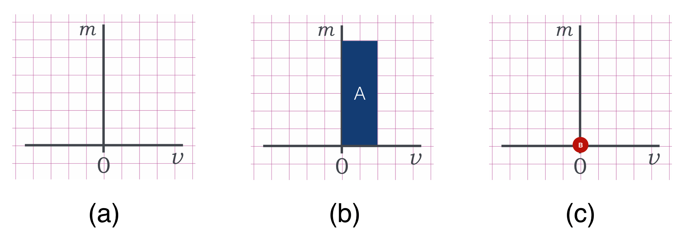
Momentum here is the product of $m$ and $v$ which is of course the area of the rectangle. For $A$ we add up the boxes and get 12 boxes, $p_0(A)=12$. The circle represents zero area and so $P_0(B)=0$
After the collision, our situation became this:
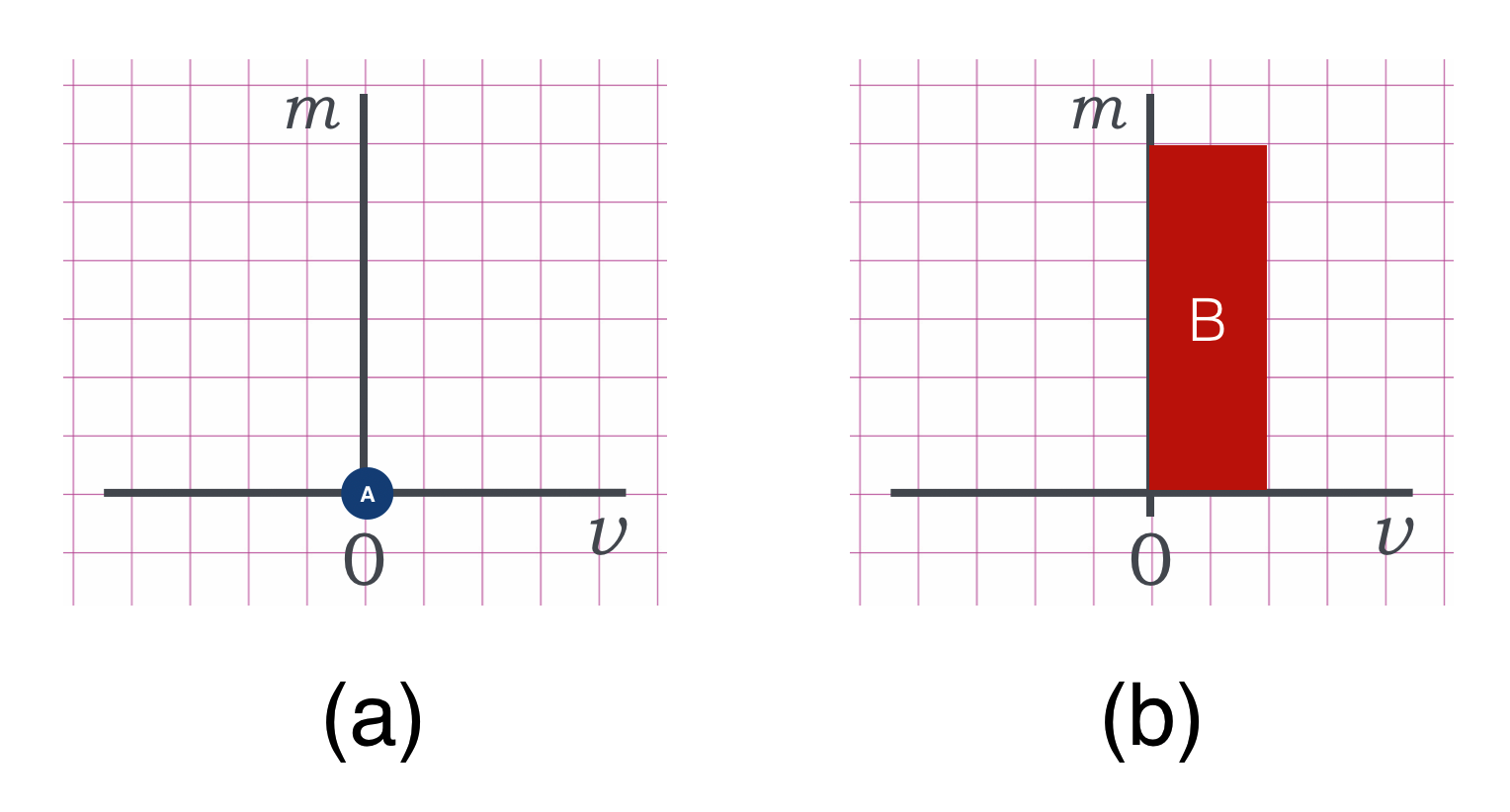
You can see that the momentum has just changed places so that the area called $B$ here is the same 12 boxes as in the previous diagram for $A$.
Momentum as thermometers
Here’s another way to represent this same situation, now dealing only with momentum.: we’ll call these “thermometer graphs.” The lengths of the “thermometers” are momentum and the directions matter: up is a positive momentum and down is a negative momentum. For our simple stop-shot, the situation is pretty straightforward:
🖋
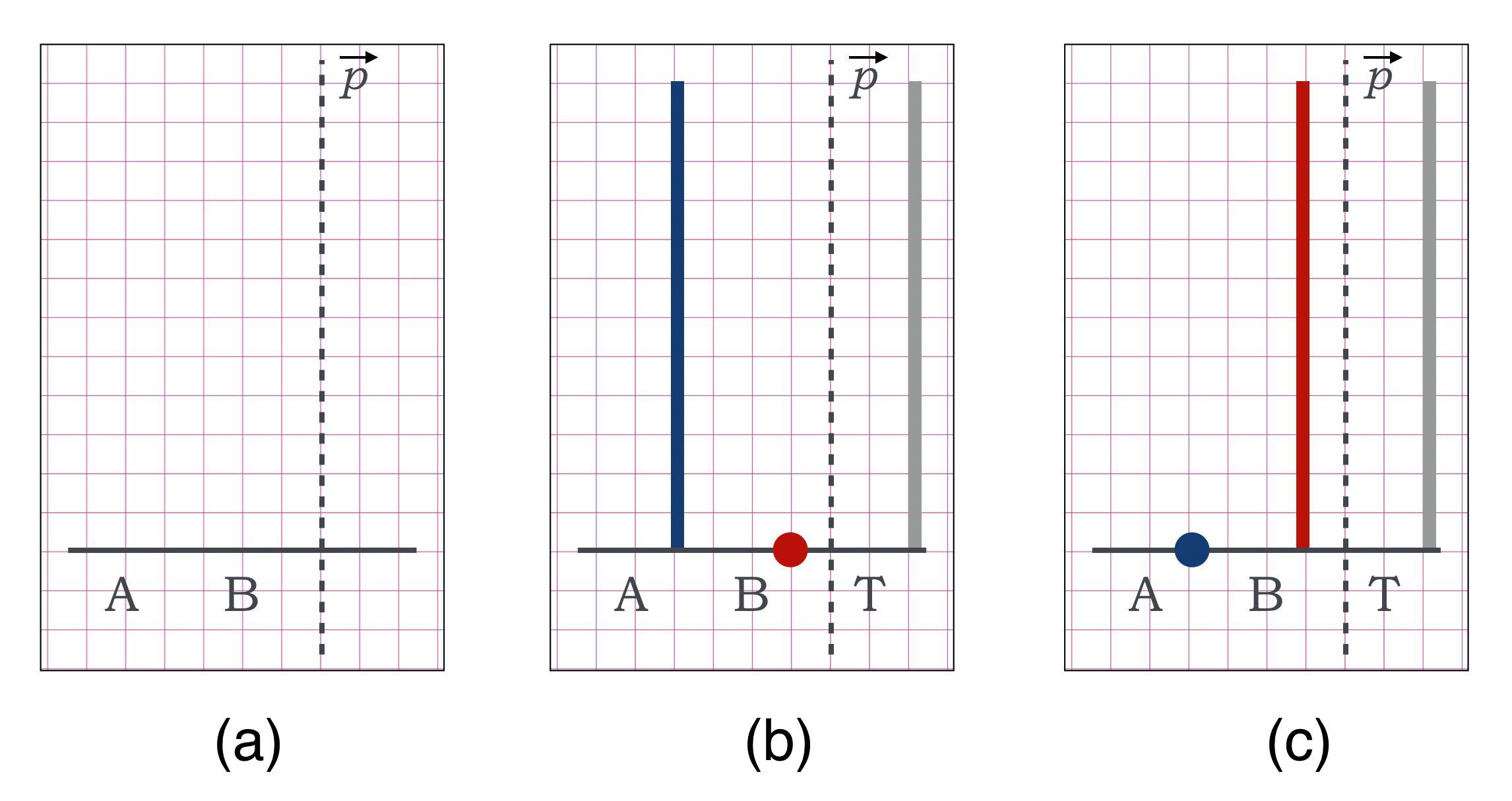
(a) sets up the working areas of the thermometer diagram. The vertical units are those of momentum. The horizontal positions just label the players (on the left) and the momentum tally (on the right). Here’s how I would reason this through.
- On the left of the vertical dashed separator line, I plot the momenta of each of the colliding particles. $A$ had momentum 12 and $B$ had momentum zero.
- Then I tally up the total momentum of the particles in the initial state and record them in a momentum thermometer on the right of the dividing line labeled “$T$” for Total.
- Then I construct the final situation where now I’m guided by the Total momentum, right hand thermometer as the final $A$ and $B$ thermometers have to add to that $T$ value.
- (c) is the result. The situation already gave us the answer since we saw it in the movie: the final momentum of $A$ is zero (stops dead) and since its momentum and $B$’s final momentum must add to that right hand $T$ momentum, we must assign the $B$ thermometer to be 12.
This is a simple problem, but a more complex problem might lead you to make a prediction based on preserving that right hand $T$ total.
Let’s do one more. The stop shot example was intentionally simple and I appealed to your experience (and a video) to tell you the result. Here’s a different situation: we’ve got a small guy moving fast, colliding, and bouncing off a large guy moving slower. Sounds like football. Let’s conserve momentum.
🖋
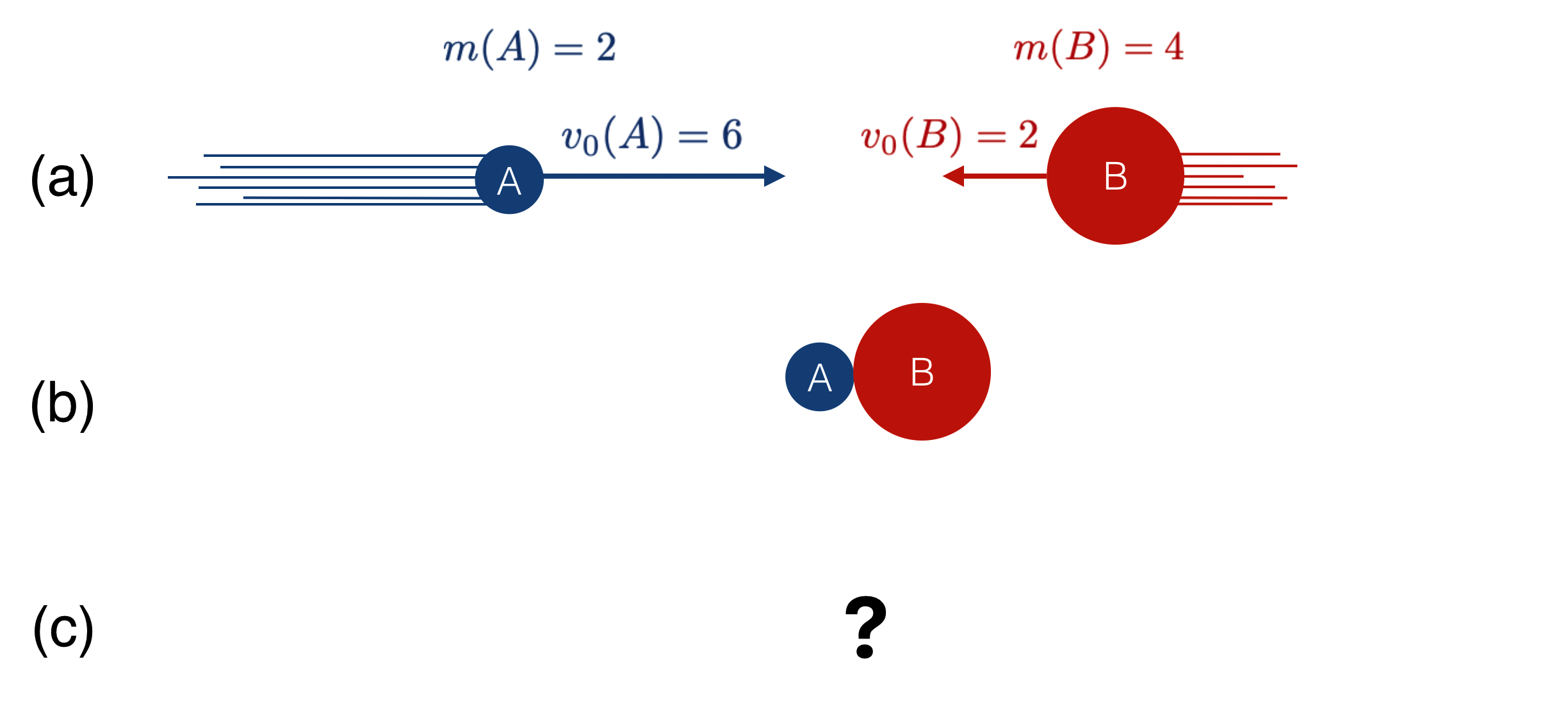
This can be Jeff ($A$) the slight, but quick football safety trying to tackle Delbert ($B$), the huge running back. Jeff bounces off the lumbering Delbert. (It could also be a small car and a large truck, but that’s too scary.)
Here is the situation:
- $m(A)= 2$ and $v_0(A)=6$
- $m(B)= 4$ and $v_0(B)=2$ the other way… so if we take $A$’s direction to be positive, then $\vec{v}_0(B)=-2$, or since we’re in one dimension, $v_0(B)=-2$
- So, $p_0(A)= 2\times 6 = 12$
- and $p_0(B)= 4\times (-2) = -8$
Of course the operative question for the defense, is whether Delbert just continues forward for a gain, or does he recoil backwards?
I’ll tell you that Jeff’s ($A$’s) final momentum is $p(B)=-9.3$: remember, he bounces back.
Here are some questions:
- What’s Jeff’s final velocity?
- What is Delbert’s final momentum after colliding with Jeff?
In order: 1. What is $A$’s final velocity?
Our intrepid (courageous!) Jeff’s final velocity is easy. We know his mass ($m(A)=2$ and his momentum ($p(A)=-9.3$), so we can get his velocity with a simple area plot:
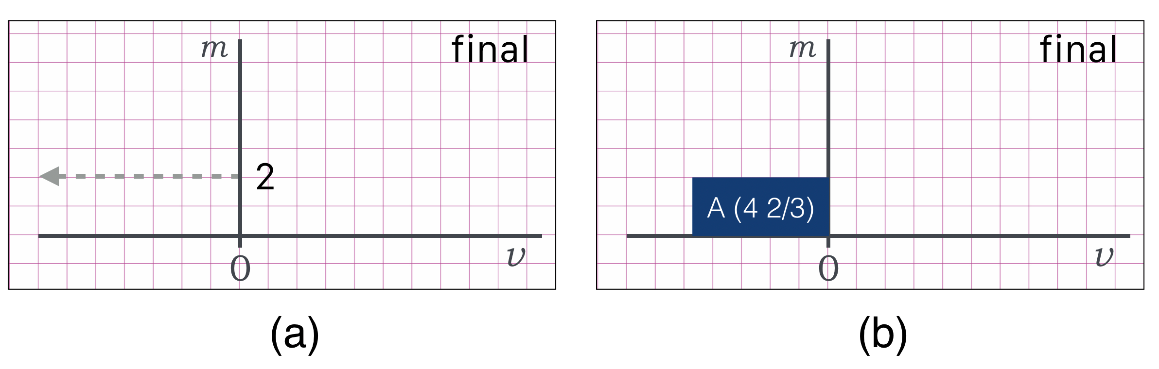
First of all, notice that this is one of those “negative areas”…the momentum is “boxed” in the negative velocity part of the graph. We can then just count the boxes until we get $9.3$ worth…that’s $4 \;2/3 = 4.67$ along the horizontal so that $2 \times (4 \;2/3) = 9.3 = p(A)$
Or, we could just solve the simple equation:
And finally: 2. What’s $B$’s momentum after the collision?
We could create areas and solve this but I think that more insight comes quickest if we use the thermometer approach. Here’s our construction:
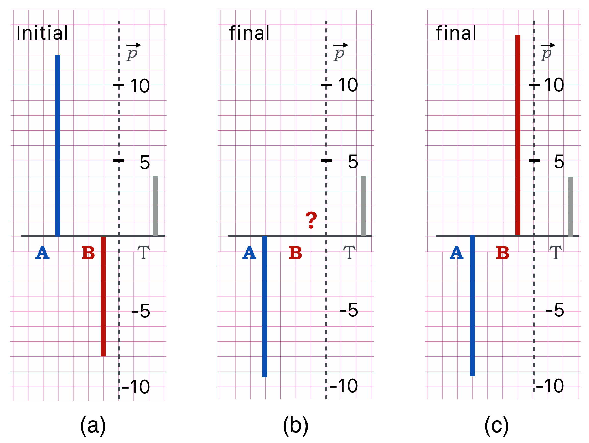
And, here’s my reasoning:
- In (a) I’ve plotted the initial momenta for each object.
- Also, I can quickly see that the difference of those momenta leave $4$, which is then the absolute total, $p(T)=4$. So the combination of the final momenta also have to sum to be that same value—momentum conservation.
- I know the final $A$ momentum, and that’s added in (b) and I brought along $T$ on the right: because THAT’s the statement of momentum conservation!
- So we can construct $B$’s momentum which, when combined with that of $A$ will give us $T$ again.
- That’s shown in (c). Count up the squares for $B$ and you’ll see that $P(B)=\text{about }13.3.$
Of course, again, with pictures I’m solving the momentum conservation equations:
Either approach is fine!
This is enough to take it our for a spin on your own:
🖥️ Please answer a question:
🖥️ Please answer a question:
🖥️ Please answer a question:
Two and More Dimensions
We will not explicitly calculate in more than one dimension, but the sorts of collisions that you’re most familiar with happen in more than one space dimension. Looking down on the pool table? The balls move in $x$ and $y$. In Demolition Derby, the cars scatter all over the infield. A pitch that’s precisely horizontal as it passes home plate, is lofted into the air in collision with the bat. We could calculate the consequences of all of these kinds of two and three dimensional collisions, but we won’t. We’ll draw pictures.
In our previous considerations of apples and billiard balls colliding, we assumed that they had no size — point-like. But striking a billiard ball precisely on its center line with a cue ball is tricky. More likely is that they would strike just slightly off-center. In that case, if we define our $x$ axis along the direction of the beam-ball, the target and the beam will both scatter into the $y$ direction. Momentum conservation helps to determine the outcome.
The most general statement of the momentum conservation rule is:
This is really a symbolic statement — a mathematical paragraph if you will – not one you can actually do algebra with. Embedded in it are two (or three, if three dimensional space) “real” equations that you can actually manipulate. In our situation that vector “paragraph” stands for two equations:
one for the $x$ direction and another for the $y$ direction. These can be separately manipulated as regular equations and you can see perhaps that overall momentum conservation means:
Momentum is separately conserved in both the $x$ direction and $y$ direction.
Momentum conservation has to hold separately in each of them but we’ll not actually solve the equations themselves. Rather, we can construct two separate Thermometer Diagrams and the transfer the result to the Momentum Diagram. We can draw conclusions without doing any algebra.
Let’s put together a momentum diagram for this situation using our arbitrary units with the following parameters to start with.
Pool balls? That’s for children. We’ll throw bowling balls at one another at twice the optimal speed for sane bowling, about 30 mph.
I’m going to use the language of “beam” and “target” here, as that’s more to our EPP liking. (In our previous collisions, $A$ would have been the beam and $B$ would have been the target.) So, now $A$ will mean beam and $B$ will mean target. Sorry that “beam” starts with B rather than $A$.
Here’s the situation.
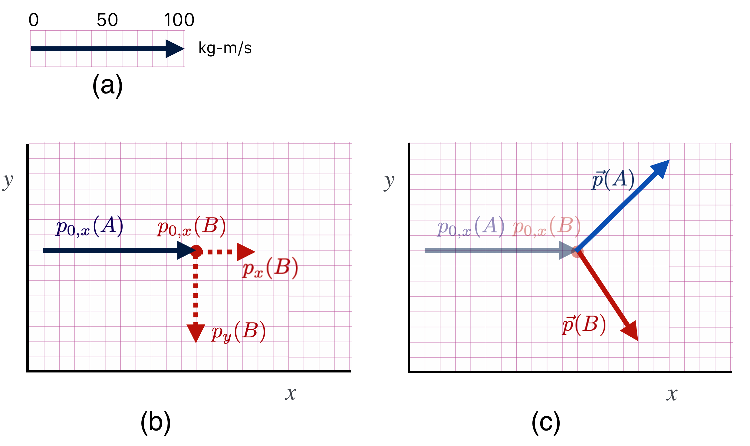
🖋
We’ll use real units here: mass is in kg, velocity is in m/s, and so momentum units are kg-m/s.
- mass of the beam ball, $A$ 7 kg
- mass of the target ball, $B$ 7 kg
- speed of the beam ball: $v(A) =14$ m/s
- so, the initial momentum of $A$ is $p_{0,x}(A) =(7)(14)=100.8$ kg-m/s (call it about 100 kg-m/s)
- speed of the target ball is zero, so $p_{0,x}(B) = 0$ kg-m/s
- Let’s say that the target ball, $B$, scatters down as show in the picture with the components
- $p_x(B)=40$ kg-m/s
- $p_y(B) = -60$ kg-m/s
- What’s the momentum and direction of the $A$ ball?
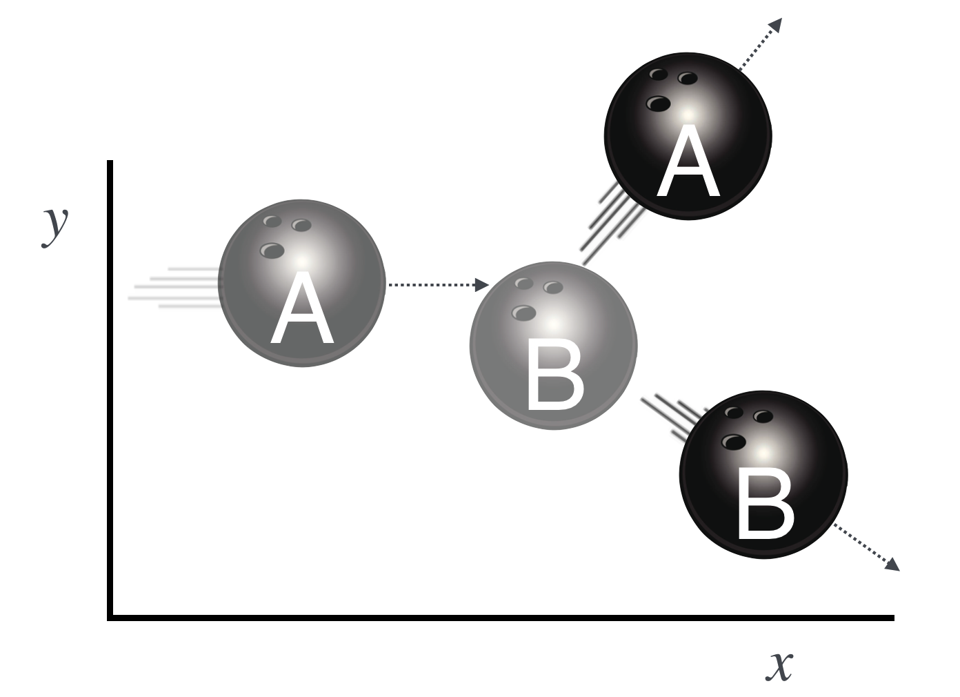
What we want to know is the momentum of the $A$ ball after the scattering. The picture sort of hints at what to expect for the direction, right?
It’s the same story as above, except we keep track of both directions separately and then combine them at the end. So here’s a picture of the initial state for both the $x$ (left) and $y$ (right) momenta:
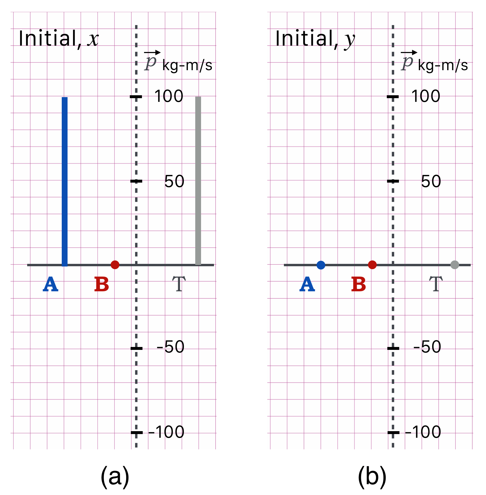
All of the action is along the $x$ axis at the beginning, so the (b) is zero. (a) is just like the stop shot in that $A$ has all of the initial momentum, in this case $p_{0,x}(A) = 100$ kg-m/s. Notice that $T=0$ for the $y$ direction at the beginning, so whatever momentum there is in the final state…it has to add to zero. Meanwhile, the $T$ for the $x$ direction is now established and carries over.
What we know about the final state is shown here:
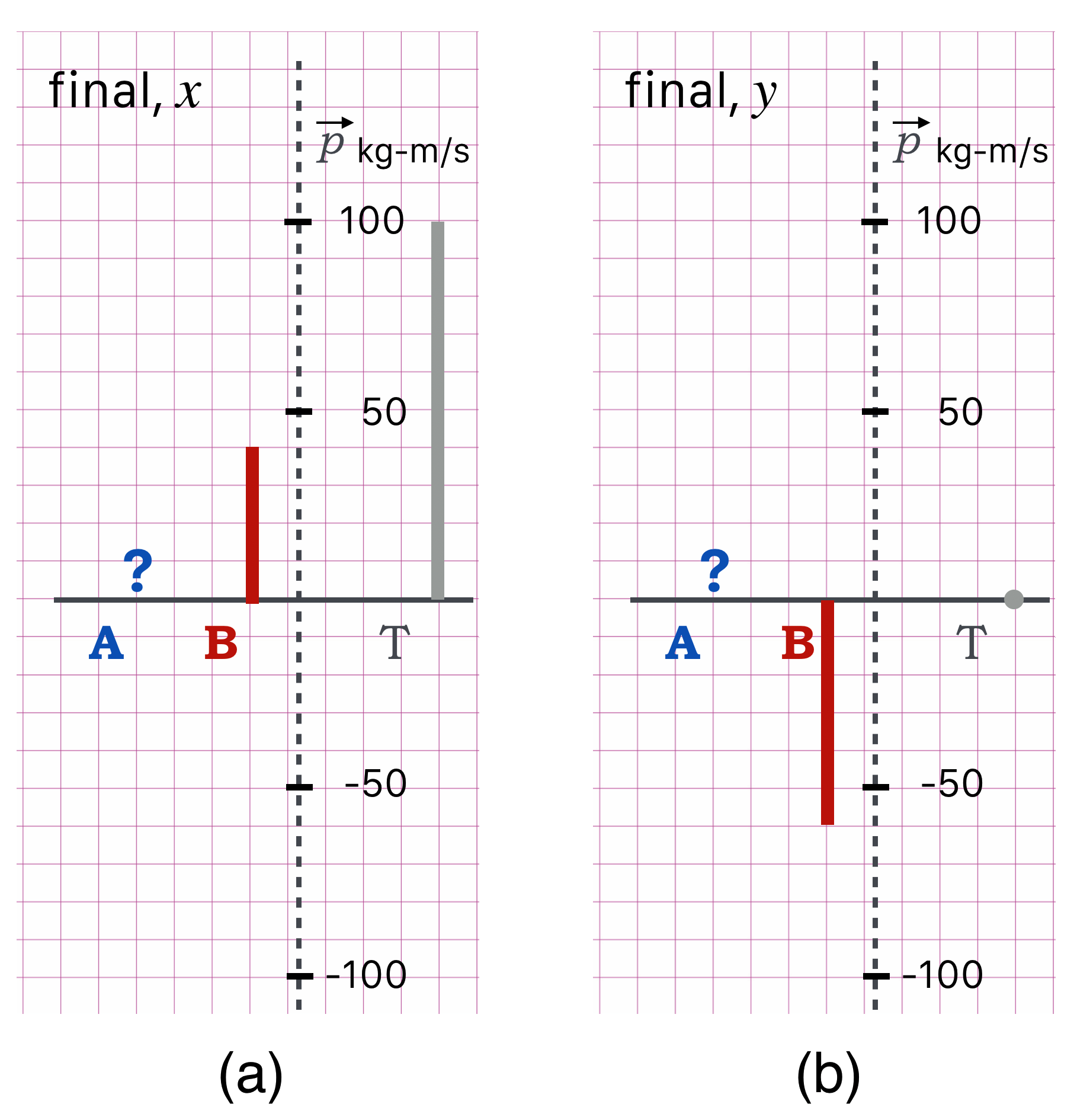
Notice that neither the $x$ nor the $y$ values of $B$’s final momenta are equal to $T$ in each direction…but momentum conservation says that they should be. So we can construct the missing $A$’s momentum:
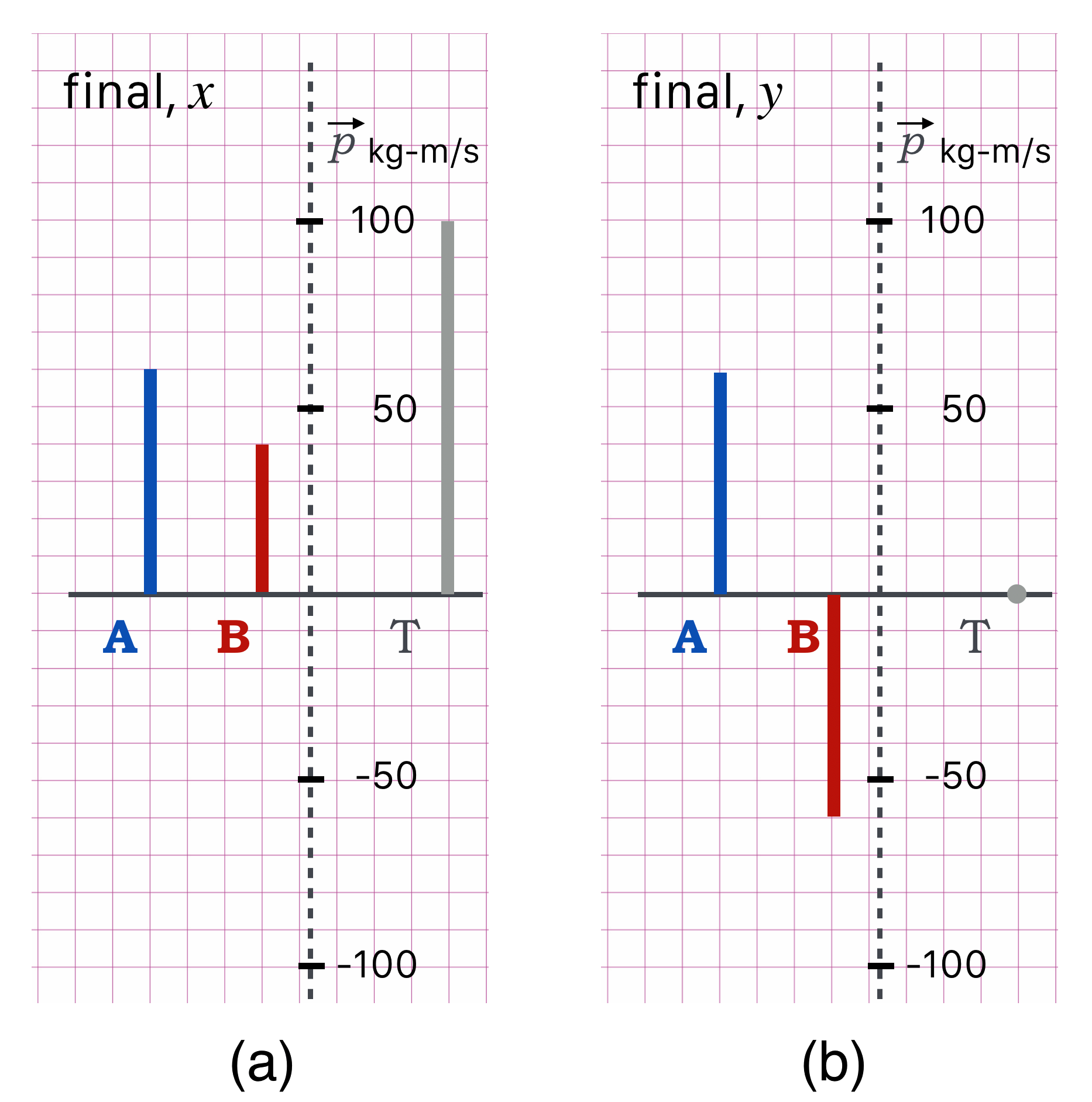
Now we know everything there is to know about the final bowling balls’ two final state motions. We can then draw a precise and accurate Momentum Space Diagram from this information:
If you followed this! You know all you need to know about momentum conservation as it pertains to particle physics (or high-energy bowling). Look at the (c) picture in the Momentum Space diagram…that looks like a Feynman Diagram and sometimes such sketches can stand in for the more formal Spacetime Diagrams. The context will tell us when to think Spacetime and when to think Momentum.
Collisions At the Large Hadron Collider
Finally, for particle collisions at the LHC two protons are precisely aimed at one another and caused to collide into lots of stuff…some of which might be other protons, but most of which is not.
Wait. Two protons? 10 Billion Euros for two crummy protons?
Glad you asked. Well, not exactly. The LHC proton beams come in about 3000 bunches of protons, one after the other 25 nanoseconds apart, in which each bunch contains about 120,000,000,000 ($1.2 \times 10^{11}$) protons. The bunches are about 30 cm long and 0.000016 meters (16 microns—a strand of your hair has a thickness of about 50 microns) across and they’re all traveling at 0.999997828 times the speed of light. Of those bunches, there are about a half-billion collisions per second. So, lots of protons collide at the LHC. We’ll learn about this later. In spite of that kind of collision mess, we can isolate individual proton-proton collisions because our electronics is really, really fast and smart. (We build some of that electronics at Michigan State.)
You now can search for new particles at the LHC. Here is an image of a collision between two protons which, because quantum mechanics is weird, will more likely produce things that are not protons. Even things much, much heavier than protons. (Mr Einstein is in the green room getting ready for his appearance in a few lessons…)
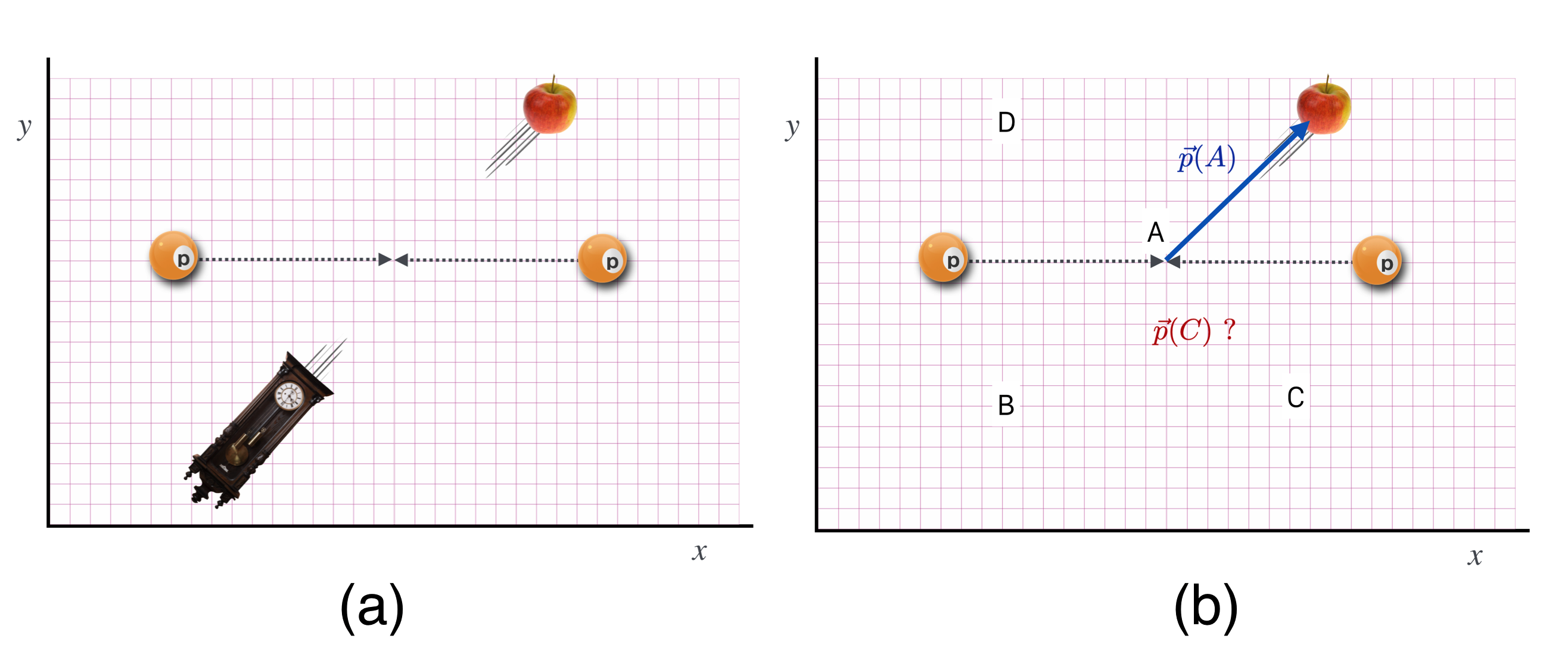
Suppose we missed the clock. We might find it by knowing what its momentum is. On the right is a measurement in which the momentum of the apple, $\vec{p}(A)$ is precisely measured ( for this example a pretty unusual detector) and is shown as the blue arrow in (b), now a Momentum Diagram.
What’s the momentum of the clock? Is it a vector from the collision point to A, B, C, or D?
Wait. I suspect it’s B, right?
Glad you asked. Sure. The momentum of the clock has to be back to back to the momentum of the apple if that’s all that is produced in this collision.
Why? Momentum conservation is at work.
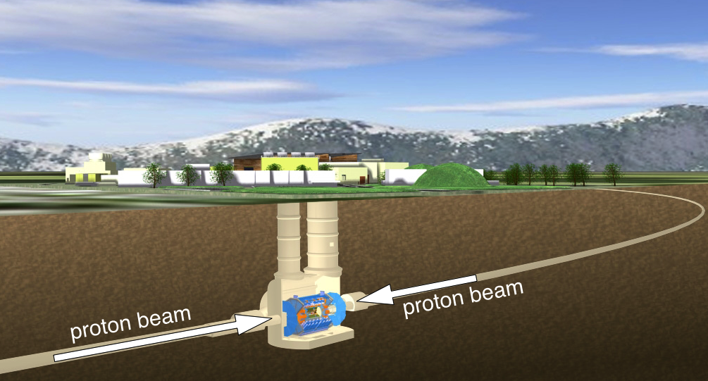
Now let’s look at some actual collisions in our experiment at CERN. This cartoon shows a a slice through the Swiss countryside where two beams in a 17 mile circumference proton accelerator collide in the center of our ATLAS1 detector. The whole operation is 300 feet underground.
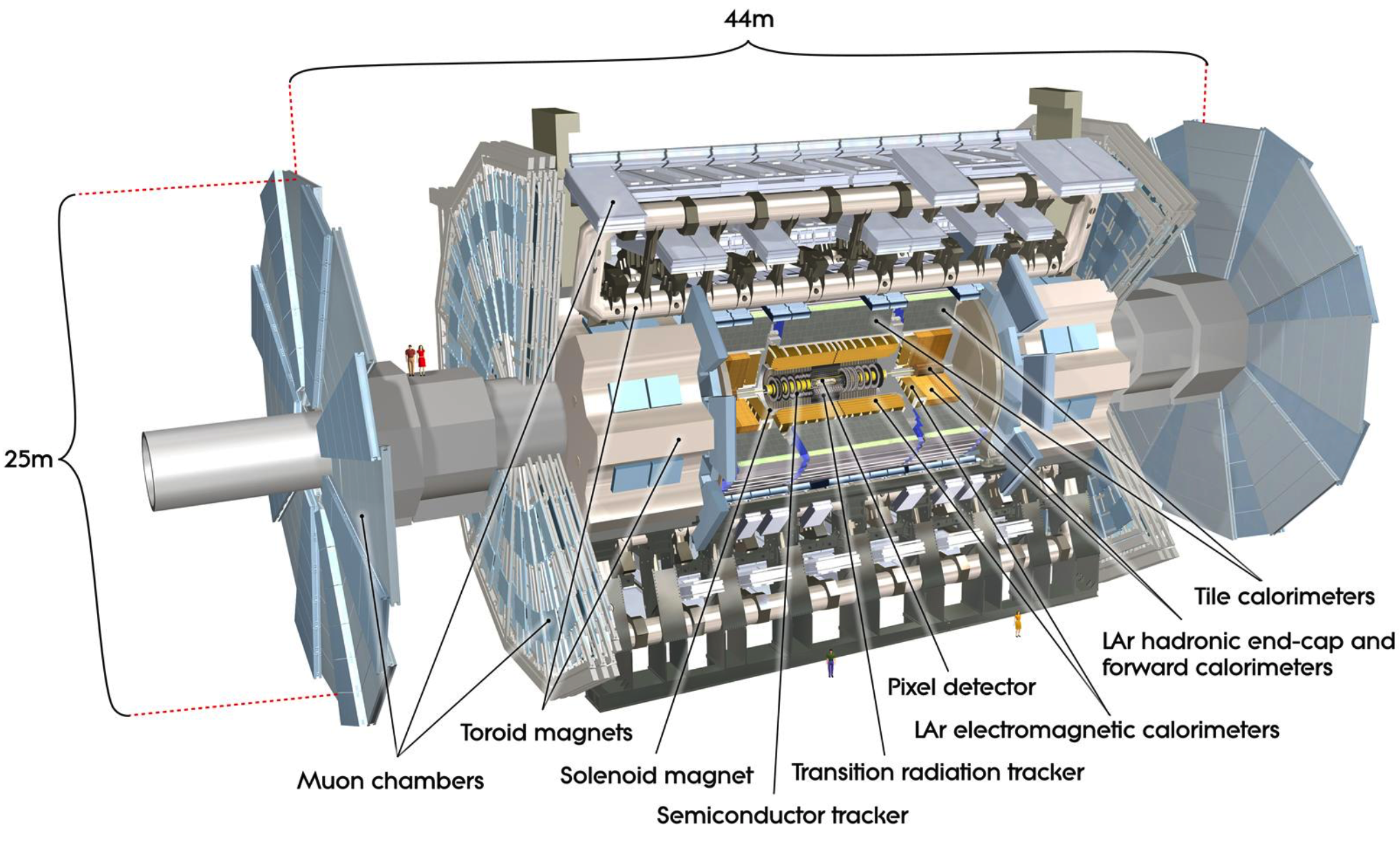
It’s useful to think of our particle detectors as concentric circles of instruments centered on the beams and the collision point. Each layer detects the presence of aspects of the particle debris that is produced when these high energy protons collide and convert their energies into matter. Here is a cut-away view of our ATLAS detector. You can see two MSU-sized people standing on the left part of the detector. It’s pretty large.
Here is a side view slice of these layers in which the protons come in from opposite directions and are directed to collide in the center.
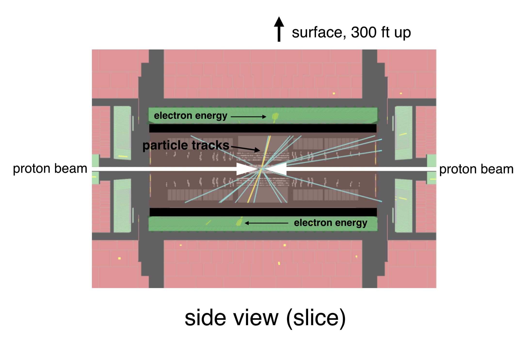
The interior red portion detects just the tracks that particle create—the computer reconstructs them into lines. The green bands (are really cylinders, but are bands in this sliced view) include detector elements that cause any electrons (or photons) to deposit all of their energies. The computer reconstructs that deposition as “blobs” that represent the energy where the electron gave up the ghost. You can see the colored tracks and the yellow blobs of electron energy-deposition.
We can also look at the detector from the end view where the beams go in and come out of your screen.
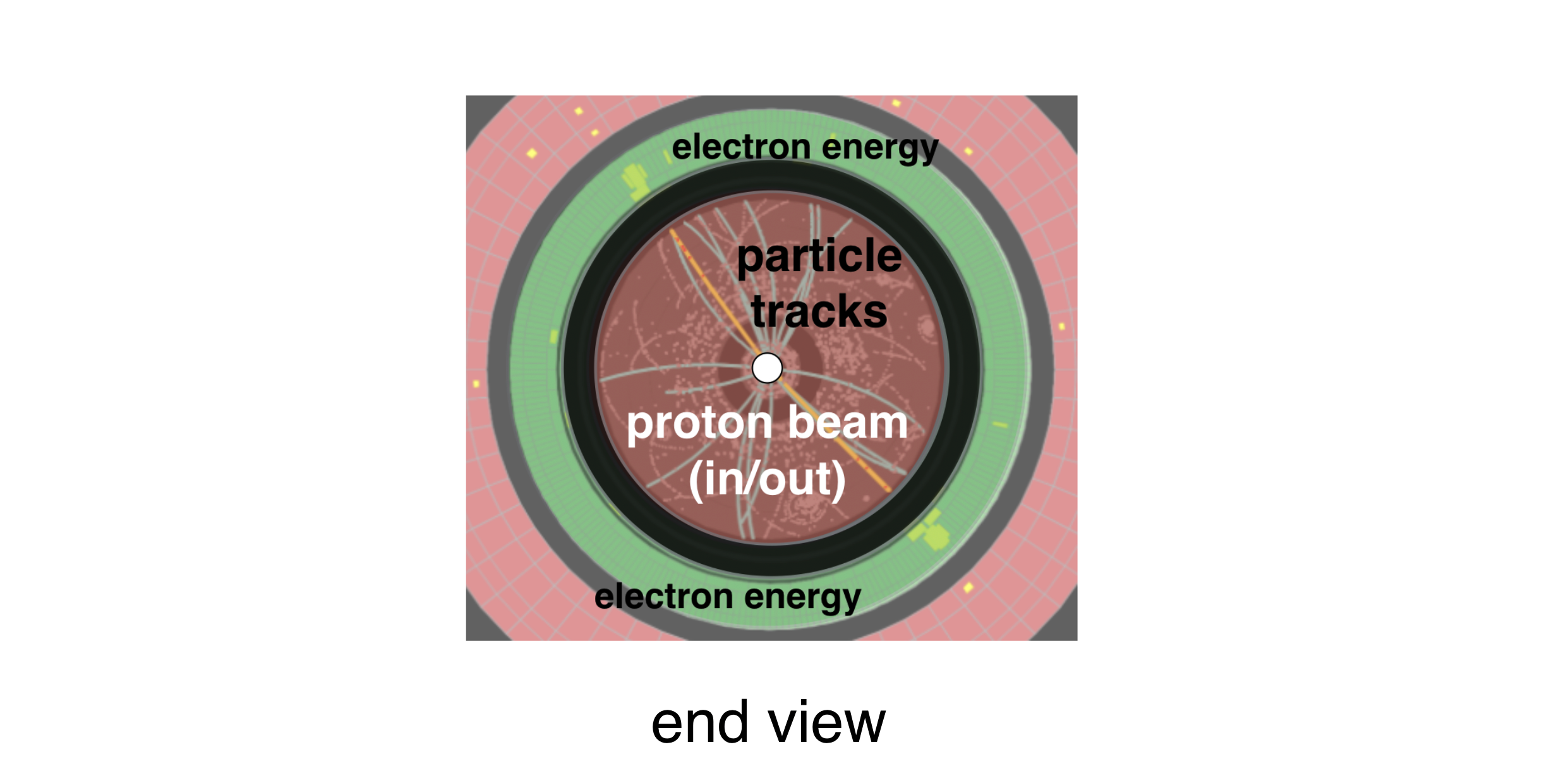
Think about the initial and final states of a collision in these monsters. The protons come from opposite directions at the exact same speeds. So, same mass, same speeds, head on—so opposite momentum vectors that cancel perfectly horizontally. Likewise, the beams are perfectly horizontal and so there’s similarly no momentum in the vertical direction in the initial state. What about the momentum components in the final state of all of the particles that are produced?
They must cancel when all added up.
Here are then some real proton collisions from ATLAS. Remember, these are reconstructions of momenta, positions, and energies of particles that a computer (actually, thousands of commodity computer cores) has turned into images for our enjoyment. The actual analysis is done on the raw electronic signals.
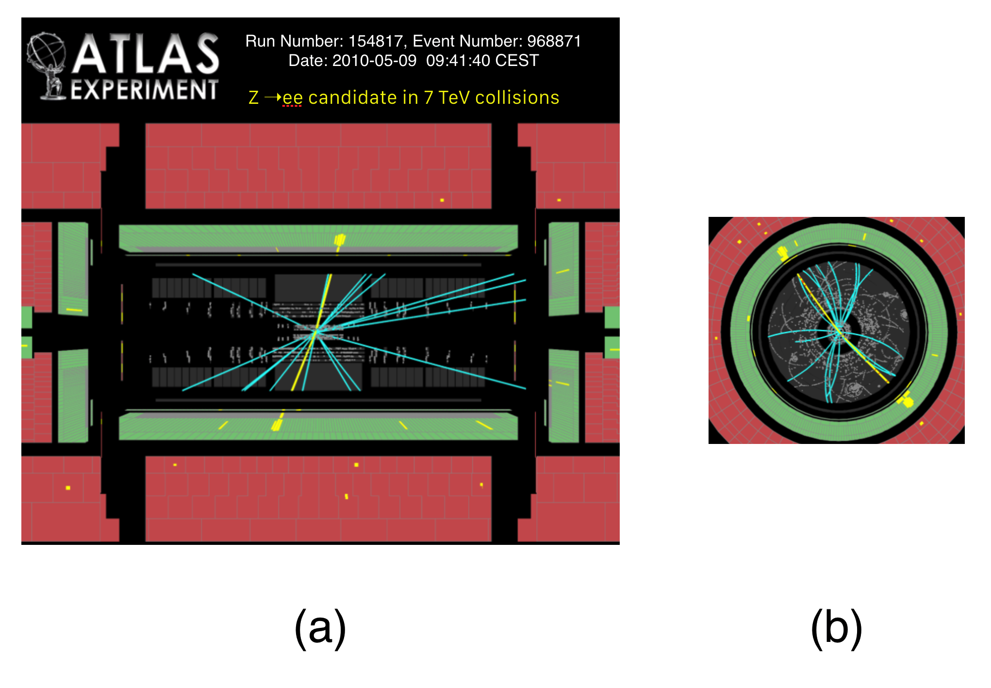
A collision has happened and it is one in which two protons collide head-on right in the center—one beam from the right and the other from the left and produce, in this case, two electrons that emerge and leave their traces in our detector as the two blotches of yellow color. You can almost think of the yellow lines and little blobs as the momentum vectors for the outgoing particles from the collision.
In the left hand picture, you seen one electron headed up and to the right and balanced by the other, down and to the left. In the end-view, those same electrons are back to back again, with the projections of their deposition shown to us. This end view is particularly useful since the initial state momentum around the beam is zero, so the momenta of the two electrons each have to be conserved in the horizontal and vertical directions. The amount of color in the “blobs” is a good measure of the magnitude of the momentum in each electron, and again, by eye on the side and the end views you can just about see that they are equal and opposite.
This next figure is a completely different situation! In scientific-speak: count the blobs. There’s only one!
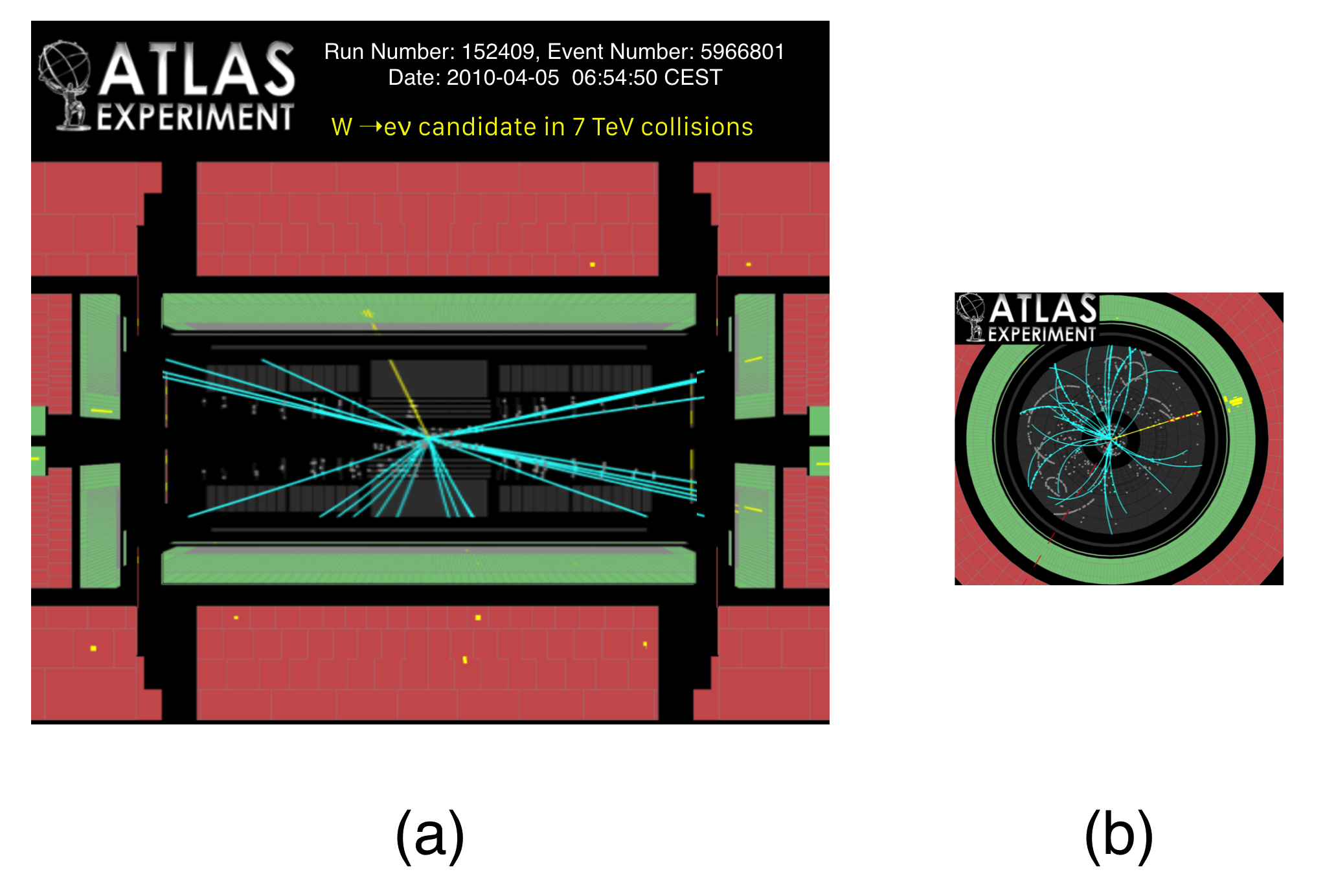
Either one of two things is likely the case about this event:
- The detector is broken. That sometimes happens, but very, very rarely and we monitor it all the time for dead regions that don’t respond.
- Some particle was produced and carries away momentum (so it balances) but it’s a particle that doesn’t interact with the material in the detector so it’s invisible.
- I lied. Here’s a third logical possibility: momentum is not conserved in this collision.
Wait. You’re messing with me.
Glad you asked. Well, sort of. But I’m making a point here. A good experimental physicist will always worry about #1. In fact, there’s never been a discovery of something unexpected in which broken or misbehaving measuring equipment wasn’t first blamed. #3 is logically a possibility, but momentum conservation is one of those rules that we’ve learned to trust very well. It’s never let us down. And even when it looked impossible (we’ll encounter that level of frustration later), it’s always recovered. So #3 is not likely at all.
In fact, #2 is the case, at least in this event. It’s our clue that a particularly elusive particle called a neutrino was produced along with the electron, and we would even say, “Look, there’s a neutrino in that event.”
Wait. You mean that you observe this neutrino-particle by…seeing nothing?
Glad you asked. We have to make such discoveries on a statistical basis. We know the rules for producing the “normal physics” that involve neutrinos and if there are other hypothetical particles that are produced, then we’d have to see them behave differently, but only after comparing many, many collisions. A statistically significant anomalous behavior can be a major discovery!
📺
Go to 6.7_2d_v1_w0m for a more in-depth discussion of these issues.
Have you got enough energy to learn about energy?
First, let’s review.
What to Remember from Lesson 6?
Momentum Conservation
The big idea of this lesson is one that will be with us for the whole of QS&BB: in any process the momentum of the constituents at the beginning of the process must equal the momentum of the constituents after the process. In one dimension, restricting ourselves to a process involving two objects, $A$ and $B$, this means that nature always arranges that
Much of this lesson tried to illustrate this in a variety of different collisions.
If the collision happens in two dimensions, then momentum is conserved along any directions one wants to choose. We typically use $x$ and $y$ directions, so nature would arrange for two conditions to be satisfied
We’ll not solve any two dimensional momentum equations in QS&BB, but we will sometimes ask what might happen in some collision and because you’re now comfortable with the idea of momentum conservation, you’ll be able to answer. Without a calculation.
-
Michigan State University has been working in the ATLAS collaboration at CERN since the middle 1990s. We have built many pieces of the detector. ↩︎