4.3. Functions, the QS&BB Way

The language of physics is mathematics, uttered Galileo a long time ago (although he said that the language of the universe is mathematics). Well, he was right. And we have no idea why that seems to reliably be the case!

“The miracle of the appropriateness of the language of mathematics for the formulation of the laws of physics is a wonderful gift which we neither understand nor deserve. We should be grateful for it and hope that it will remain valid in future research…”

This is from the last paragraph of a notorious and actually delightful essay written by the physicist Eugene Wigner in 1960. The title is The Unreasonable Effectiveness of Mathematics in the Natural Sciences, where he tries to dig into the strange relationship between the physical world and mathematics. It’s famous: ask Mr Google to find “Unreasonable Effectiveness” and you’ll get 150,000 references to Wigner’s essay.

I'll go further and suggest that a mathematical model cognitively---you know, in your brain---functions similarly to how a painting represents the object of its representative landscape. Functional MRI investigations suggest that mathematicians and physicists appreciate beauty in mathematics by heating up the same region of the brain that's stimulated by someone appreciating a work of art. So this is deep stuff.

I hope you see my point: The English paragraph and the succinct mathematical function do the same job, on the surface. However, that “miracle” of the connection between the universe and mathematics is really only apparent when we make full use of the manipulative features of symbols in an equation where we can uncover new things.

4.3.1. Functions rule

One of the remarkable consequences of the mathematization of physics that began with Descartes is that we’ve come to expect that our descriptions of the universe will be in the language of mathematical functions. Do you remember what a function is? The fancy definition of a function can be pretty involved, but you do know about function machines and I’ll remind you how.

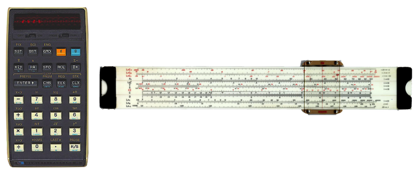
When I was a senior in college, finishing my electrical engineering degree, our department had a visitor from the Hewlett Packard Company. It was either Bill Hewlett or Dave Packard, I can’t remember which. But he promised to do away with the slide rule that we all carried around with us everywhere and showed us a brand new product: a portable scientific calculator, that they called the electronic slide rule. This was 1972 and he showed us the first HP calculator, the HP-35. Needless to say, I couldn’t afford it—it cost $400 then— but later in graduate school I bought my first scientific calculator, the HP-25, pictured here, along with that slide rule that I carried for four years.

Left: the venerable HP-25 programable (!) scientific calculator. Right: a slide rule used for all calculations until the early 1970’s. It was not programmable (although it was wireless)

Today I’ve got more processing power in my watch then I had in that calculator. But I’ll bet you’ve got something like it…calculators are nothing but electronic function machines. In fact, this is the arithmetic circuit inside of that original calculator:

The AMI 1820-1523 Arithmetic, Control Timing processor: the heart of a function machine. Adapted for my silly purposes: the tabs at the blue arrows are actually connecting the processor to the keyboard. That’s how data got in.

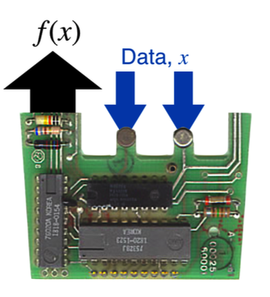
The calculator guts shows what a function does: if you enter data through the keypad — a value of \(x\) — and hit the appropriate button, the display shows the value of the function. So if the function was the formula \(f(x) = x^2\) and if I keyed in “4” and pushed the \(x^2\) button, the display would read “16,” the value of \(f(4)\) for that particular function. Notice that it doesn’t give you more than one result, and that’s a requirement of a function: one result.

That’s all a function is: a little mathematical machine that reports a single result for one or more inputs according to some rule. For us, functions can be represented by a formula, an algorithm, a table, or a graph. In all cases, it’s one or more variables \(x\) or \(x \; \& \; y...\) or \(x \; \& y \; \& z...\) inside, of a rule about what happens to them, and one numerical result out.

Nature seems to live by functions and since we’re all about nature, we’ll need to use functions. Our way.

4.3.2. Turn the crank, QS&BB style

We’ll accomplish a lot without much mathematical effort, I promise you. In fact, we’ll find that the raw mathematics of modern physics is simple. What’s hard is the conceptual visualization.

Some physics models are simple and we can easily deal with them in their “raw” mathematical form…and some are really quite complicated. With a little help from Mr Descartes or some whimsy, we’ll manage. So three ways we’ll work with mathematical models.

4.3.2.1. We’ll write them and manipulate them for real.

Can you solve the equation: \(y = ax\) for \(x\)? You’ll be surprised just how often an equation of that form will describe sophisticated aspects of the world.

4.3.2.2. We’ll Plot them.

If I want to deal with a model that uses sophisticated mathematics quantitatively, instead of working with the formulas…I’ll just show you the functions are plotted. Here’s an example, a really important model in physics which we’ll refer to a number of times. The function is messy and I don’t want to lose track of the physics by getting you bogged down in evaluating the it.

This is the intensity of a heated object as a function of wavelength of the radiation for different temperatures (noted in units of Kelvin).

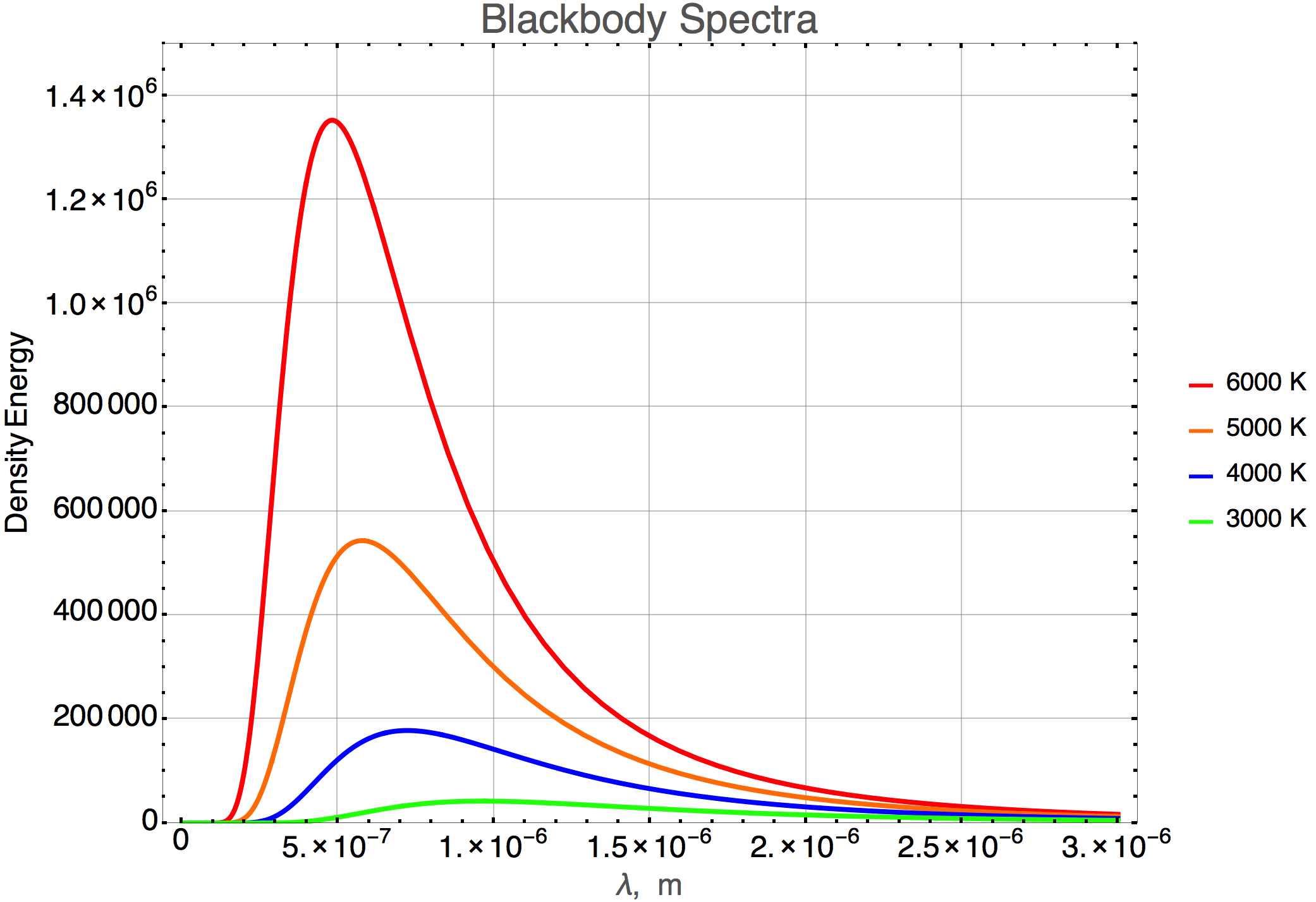
You’d have no problem telling me the relative intensities of say the blue and the red curves—4000 degrees and 6000 degrees—at a wavelength of 1 micron, \(1 \times 10^{-6}\) m. Right? Much easier than plugging into Mr Planck’s formula.

4.3.3. We’ll represent with a circuit. A silly circuit.

If we’re talking about a really complicated model, perhaps one with many formulas and lots of high-brow calculus or even worse, I’ll show you a cartoon and ask you to take my word for it.

Remember in your past you might have heard someone use the phrase, “turn the crank…” that’s sort of old language for plugging in some numbers and doing some laborious calculation…. We’ll not do that. I’ll just show you this figure, properly filled out for the circumstance at hand:

The evaluation of a candidate physical model (which is a function or a set of functions) requires some inputs [the equation(s), maybe some data, some core beliefs (other trusted models),and some plan...a strategy]. The result is a prediction which would almost always be a prediction for some measurable quantity.

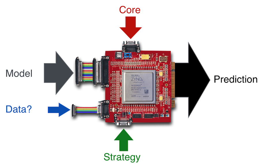
What will be important here is that we all agree on the assumptions in the model, the tools used to solve it, and any data that might be a part of the calculation of interest. You’d have no problem imagining a computer solving something or running some (game?) simulation and that’s all this fake circuit represents. Something in, some instructions, and something out. We move on.