4.6. A Gentle Review 2: Skills for Only a Few Times#
There are a handful of skills that will sometimes come up, but not every lesson. I have in mind here reading log-plots, unit conversions, approximating functions, simple graphical vector manipulations, and a few more geometrical relationships.
4.6.1. Log-Log and Semi-Log Plots#
Wait. LOGARITHMS!!? NO!
Glad you asked. Calm down. There will be only a couple of times when I’ll ask you to read a plot…meaning identify a point on a curve in which the axes are not linear (1, 2, 3, 4…) but logarithmic (10, 100, 1000…). No functional manipulations. Just interpretation.
Sometimes it will be useful to plot functions or data that range over a wide scale, maybe even many powers of 10. I want to make use of log-log plots and semi-log plots because it’s about the only way to display functions that range over many orders of magnitude. So we’ll use them as a tool, but we’ll never actually evaluate a logarithm. Here’s an example.
We’ll learn that there is a relationship between the time it takes for a planet to orbit the sun (its “period”) and the distance away that its orbit is from the center of the sun. Here it is for a slice of distances. The graph displays the orbital period in units of days versus the distance from the sun in units of 100,000,000 kilometers. So the left hand “origin” is at 100,000 km, then the next big tick mark is at 110,000,000 km and the next (labeled) tick mark is at 120,000,000 km. That’s a lot of zeros, so I labeled the horizontal axis as units of \(10^8\) km.
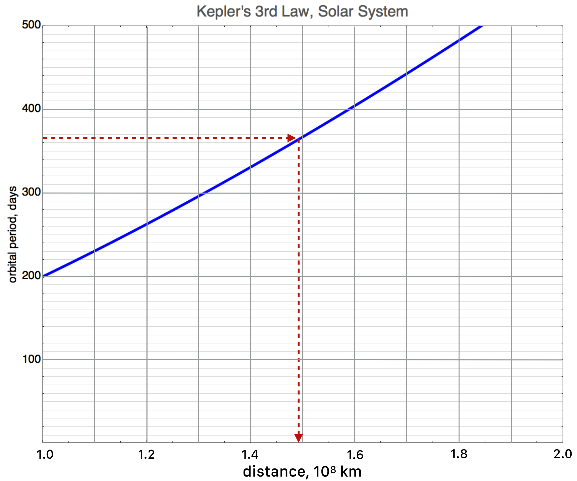
If I asked you to find the distance earth, which has a period of 365 days, is from the sun, you’d look at the vertical, period axis, dig into the tick marks, and figure out where to find 365 on the vertical axis, right? I’ve kind of done that — what your finger would probably do — and I find that the horizontal, light lines are at every 10 days and the tick marks are at every 20 days, so I’d find 365 at about where the horizontal arrow is. Using the model — solving the equation that relates period to distance — means simply finding the point on the curve and reading down to the distance. Going down from the curve, it would hit at about \(1.5 \times 10^8~\)km. That’s about right.
If I asked you to do the same thing for Venus, but the other way around you could do that.
Pens out!
If Venus is \(1.07 \times 10^8\) km can you convince yourself that its orbital period is about 226 days?
How about Mars? Its period is about 687 days. Certainly the model (the blue line) should describe Mars. How about Mercury? Its period is 87 days and it’s distance is \(0.58 ]\times 10^8\) km. How about Neptune? It’s period and distance are 60,200 days and \(44.8\times 10^8\) km. None of these fit on the graph. So this plot is pretty useless as a guide to the solar system. Don’t despair. There’s a way.
This is where a log-linear or log-log plot saves the day. In a log plot the axes are labeled by powers of 10, so 1, 2, 3… and so on, standing for \(10^1, 10^2, 10^3\). This power relation distorts the curve from presentation on a linear scale pair, but it’s not wrong, just different. Let’s do that for our solar system for the horizontal axis.
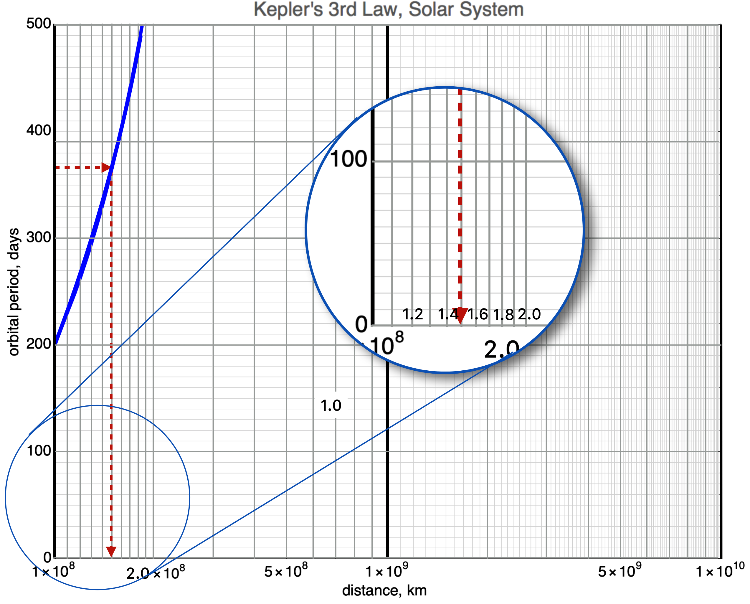
In this figure, the dark, black vertical lines tell you the \(1\times 10^8, 1\times 10^9, \text{ and } 1\times 10^{10}\) km marks. The vertical gray lines indicate the \(2, 3, 4, 5, 6, 7, 8, 9\times 10^{8, 9, \text{ or }10}\) km marks. The circular inset breaks down the \(10^8\) region to that of the linear horizontal plot up above. Notice that the red, dashed lines mean what they did in the first plot: 365 days for Earth’s period on the vertical axis and about \(1.5 \times 10^8\) km for Earth’s distance from the center of the sun on the horizontal axis.
But we still can’t represent much of the solar system in one plot, so we must also make the vertical axis logarithmic. A “log-log” plot, whereas the previous is a “linear-log” or “semi-log” plot. Here it is, the model of orbiting planets around our particular Sun. Earth is again represented as the red, dashed lines and now we can evaluate the periods and distances for many more planets.
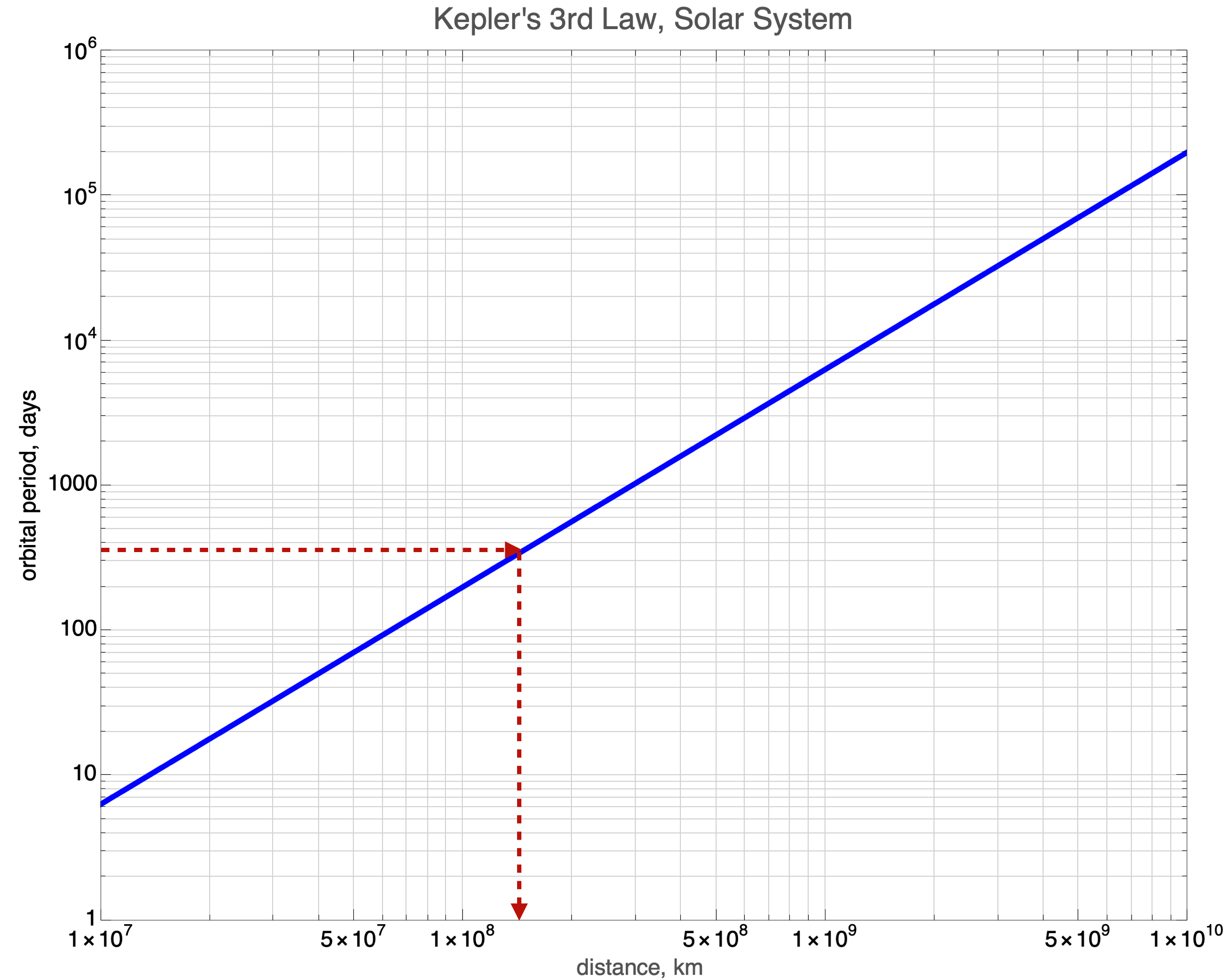
This covers 6 orders of magnitude in days and 4 orders of magnitude in kilometers.
Pens out!
Jupiter is \(483 \times 10^6\) miles from the sun. What’s its period in days? You’ll want to consult Mr Google to get km. The period is about 4000 earth days, about 12 earth years.
4.6.2. Unit Conversions#
Numbers are just numbers without some label that tells you what they refer to. Not all numbers have to refer to something, a pure number is a respectable mathematical object—prime numbers for example have been a topic of research for centuries. Irrational numbers — those that can’t be expressed as a ratio of whole numbers, like \(\pi\), — are likewise objects with no necessary relationship to…“stuff” in our world. But they keep coming up in nature, so we warm to them.
We’re mostly concerned with numbers that measure a parameter or count physical things and they come with some reference unit (“foot”) that is a customary way to compare one thing with another. Of course not everyone agrees on the units that should be used. Wait. Let me restate that: there’s THE WHOLE WORLD that agrees on one set and then there’s the United States that marches to its own set of units. Thinking of you, “feet,” “pounds,” and “Fahrenheit.”
I’ll not use Imperial units (feet, inches, pounds, etc.) very much, except to give you a feeling for something that you’ve got an instinct for…like the average height of a person or a single story house. We’ll use the metric system, in particular the MKS, aka SI units[1] in which the fundamental length unit is the meter (about a yard), the fundamental mass unit is the kilogram, and the fundamental temperature unit is the Celsius. I’ll generically refer to these as “MKS” (for meter-kilogram-second) or “metric units” without being too fussy about the fancier names, like SI.
It’s small comfort that we’re all in agreement on seconds, minutes, and hours and its base-60 origins. In 1793 the French tried to change that to “decimal time” with a 10-hour day, 100 minutes in an hour, and 100 seconds in a minute and so on, but it didn’t catch on.
Just like an exchange rate in currency, so many euros per dollar, we’ll need to be able to convert among many different units. All the time.
Wait. That can be pretty involved.
Glad you asked. You’re right and it can be a way to make mistakes and get all wrapped up in the conversion that you lose track of the physics. You know what? I’ll not care. I’ll give you little conversion engines that will do any unit conversion that you need to do. Just let me show you what it means and then we’ll be pretty low-key about this.
Having said that, we should review how this works—what will be behind any tool that does unit conversion.
Let’s get our bearings. What’s the height of an average male. Mr Google tells me that’s about 5’10”. How many inches tall is our average male? Here’s the pre-QS&BB thought-process you’d use to calculate this.
Three steps:
A single foot is \(12\) inches.
So, \(5\) feet is \(5 \times 12\) = \(60\) inches
and the combination is \(60 + 10 = 70\) inches.
…which you could almost do in your head, which, by the way, averages in circumference at about 22 inches. You’re welcome.
But this simple, almost intuitive calculation uses a more general conversion from one unit to another through a tricky multiplication by the number 1. Can you multiply by 1? Then you can convert units like a champ.
Pens out!
Here’s a cute way to write 1 by starting with some basic conversion translation like \(12 \text{ inches} = 1 \text{ foot}.\) Then you make “1” out of it:
All unit manipulations this conversion factor and all you have to do is figure out which version to insert.
Armed with this, we can do the conversion of 5 feet to inches.
Notice that we treat units like algebraic terms and can cancel them as if they were symbols or numbers: the “feet” cancel above. That’s the neat thing. If you set up the conversion factor right, the units will multiply and divide along with numbers so you can always see that you get what you want.
While this is a particularly simple conversion, sometimes we’ll need to do some which are either more complicated, or use units that maybe you’re not very familiar with. I won’t be so pedantic usually, but hopefully you get the point!
Let’s work out an example. Something you can use at a party. I first worked this out for a class when I was in Geneva, Switzerland working at CERN. It was July 4, 2010, which was just another Sunday over there. The United States came into existence on July 4, 1776[3] which was \(2010-1776 = 234\) years ago.
Pens out!
Question! How How many seconds had the United States been around if we start from midnight on July 4, 1776?
Glad you asked. We need a handful of 1’s here:
Now it’s a matter of just multiplying by the right combinations of “1” as many times as necessary to get where you want to be.
Good job!
There are a few of things to notice here. First, that’s a lot of seconds! Second (get it?), if we’d known that there are \(3.154 \times 10^7\) seconds in a year we could have started with that and had just one factor of 1. And finally…”3.154”? Does that sound familiar to anyone?
Quite by accident, the number of seconds in a year is close to the first few digits of \( \pi = 3.14159... \) times \(10^7\) and so we often say that the number of seconds in a year is about “\(\pi \times 10^7\).” Just as a memory device. You’re welcome.
4.6.3. Vectors, 2#
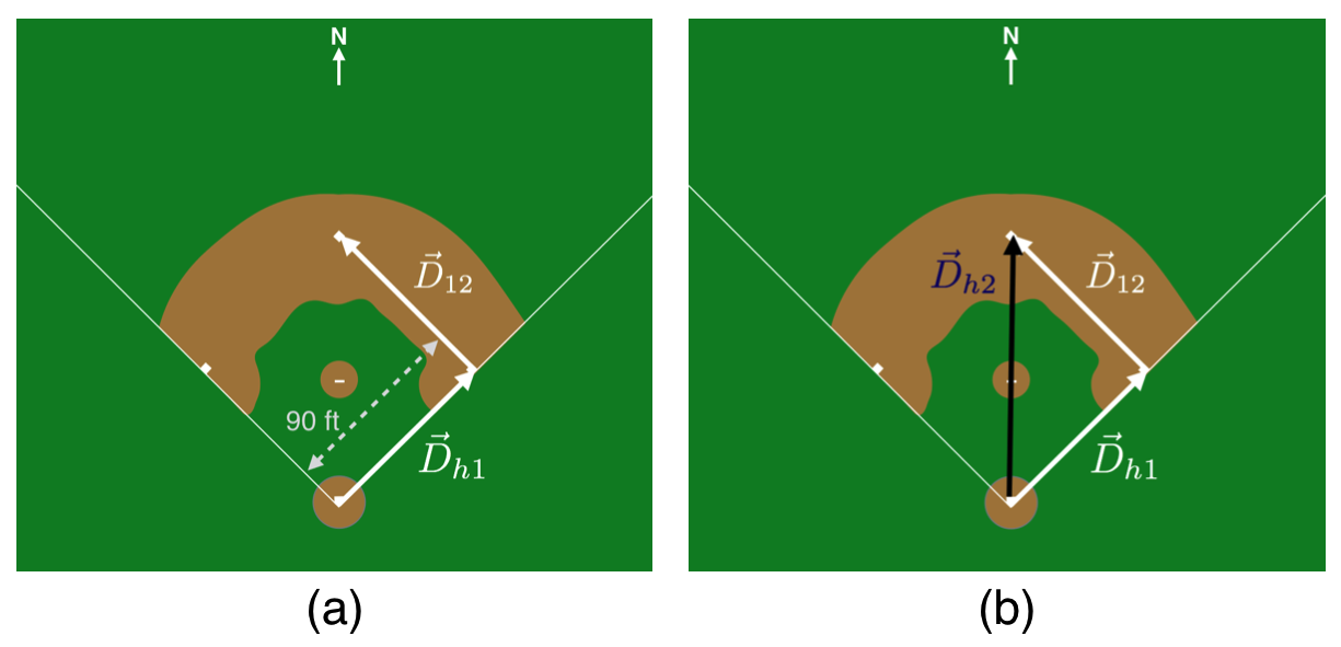
Some quantities in nature have a magnitude (like a temperature) and a magnitude and a direction, like a velocity. 60 mph north does not result in the same trip as 60 mph east, so direction and speed both matter. I think that the most intuitive vectors are those associated with a distance in space and a force, so in this survey I’ll concentrate on those two. We’ll meet many other vectors throughout QS&BB, but I’ll highlight their vector natures when we come to them. As I’m writing this, the World Series in 2018 is about to start, so let’s think about a baseball diamond.
In baseball, the distance between the bases is 90 feet and according to the rules, a runner must follow the bases in order. So to go from home plate to second base, the path that’s followed must be according to the two arrows in this figure. This situation is shown in the (a) below. Here, Frank has hit a double and being a good sport has indeed taken the appropriate path to second base.
Pens out!
Notice that the total path is represented by two vectors,
\(\vec{D}_{h1}\) and \(\vec{D}_{12}\).
There are many ways to represent the combination of magnitude and direction for a vector. When marking with a pencil, one would typically draw an arrow over the symbol as I’ve done here. In a fancy printed version, the \(D\) would be bold, D. We must also adopt a coordinate system in every situation so that the direction can be concretely specified. You might have used an \(x-y\) coordinate system, but that’s not necessary. Here the ballpark has been layed out with north being directly to second base from home plate—that’s a coordinate system.
In order to represent all of the information in a vector, we’ll be satisfied with either a graphical representation—a labeled picture—or something else. Here’s an example. If Ossie hits a single, we could represent his trajectory vector from home to first base as
The formal name for a vector in regular space is displacement and the formal name for the magnitude of a displacement vector is length or distance so the vector \(\vec{D}\) is the displacement and 90 ft is the length.
Maybe not the way you might have seen a vector displayed, but it’s perfectly okay. It encodes the length (90 feet) and the direction (northeast) in one thing.
Next up, Dewey smacks a double, and so his vector would be
Chester is up next and realizes that the shorter distance from home plate to second base is straight north across the diamond over the pitcher’s mound, which is shown in (b). While he hit the ball to the warning track, after that day he didn’t play long on that team since he took that shorter path and was called out for not following the rules. What’s okay in mathematics is not necessarily okay in baseball.
Chester is right, though. Before he was called out, he correctly navigated what is actually the vector sum of two vectors:
Both the left side and the right side of that equation are equivalent in that they both connect home plate with second base.
Pens out!
Question! Earlier Earl was at bat and hit a ground ball to the shortstop but he fell down halfway to first base. How does his displacement compare to Ossie’s in vector notation?
Glad you asked. Before his embarrassment, Earl was running in the same direction that Ossie ran—and thousands of ball-players before them. However his vector would be:
an arrow pointing from home plate halfway to first base.
Good job!
Dewey was also unlucky and after Chester was called out he tried to steal third base from second base, but fell down 1/3 of the way. What’s the vector that represents his short trip?
In QS&BB we’ll make a lot of use of the handy arrow symbol: \(\rightarrow\). The length of the arrow represents the magnitude and of course the orientation and the head of the arrow represent the direction. Arrows can be \(\longrightarrow\), or short \(\rightarrow\), pointed in different directions, \(\nwarrow\), \(\leftarrow\), \(\nearrow\), etc. Very handy.
The magnitude can mean many things, depending on the physical quantity being represented. Some of the vectors that we’ll meet are displacement, velocity, momentum, force, electric field, magnetic field, and angular momentum.
A few useful things from this figure:
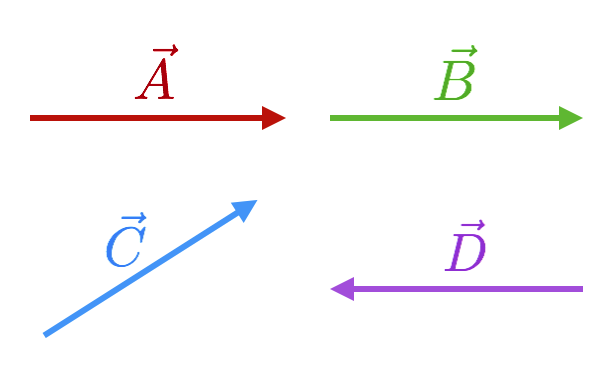
Two vectors, \(\vec{A}\) and \(\vec{B}\) are said to be equal if they are both the same length and point in the same direction so
Vector \(\vec{C}\) is the same length as both \(\vec{A}\) and \(\vec{B}\) but
because its direction is different. Finally, the negative of a vector is that same vector pointing in the opposite direction. So for example,
4.6.3.1. Vector addition in one dimension#
Generally, we’ll treat a vector quantity as an arrow pointing in some direction and a length that represents its magnitude. Sometimes a vector can represent an actual path in space (like meters, feet, and so on) where it’s easy to imagine what it means. We do this all the time on maps with a scale showing that some map-distance (an inch) can stand for a real-world distance (“1 inch = 1 mile”).
But, sometimes a vector doesn’t represent a length in space, but some other physical quantity, like a force or a velocity. This can be complicated since you’re drawing an arrow that has a “regular” length, but you mean it to be something else, like a force. But, it still works geometrically (the arrow still points in space) and we just use a different scale. Let’s do something simple.
Pens out!
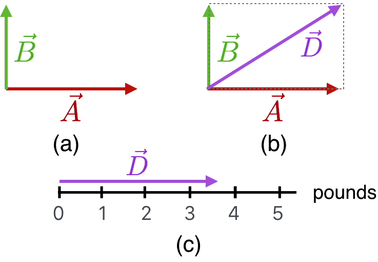
In the next figure are two vectors that now represent forces, so their lengths have the units of pounds. I’m obligated to provide a scale and you can see it. Vector \(\vec{B}\)’s length has a magnitude of 2 pounds and \(\vec{A}\) is one pound more.

If \(\vec{A}\) corresponds to Muriel pulling the leash on her reluctant and enormous dog and vector \(\vec{B}\) corresponds to Earl’s ability to also pull, then the two of them together can pull with the obvious 5 pounds.
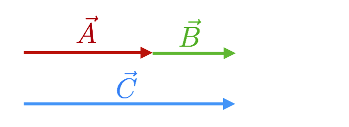
This is our first vector addition problem. The total vector force that the two of them can exert is in pictures above and in symbols
Here’s the rule: We constructed \(\vec{C}\) by connecting the tail of one vector with the head of the other. Keep that in mind, even though it’s pretty obvious when everything is along one direction.
4.6.3.2. Vector addition in two dimensions, the head to tail way#
Here’s a different combination of vectors, which looks more like Chester’s baseball career’s embarrassing final act. Here, we have two vectors that have the same lengths on your screen, but now their lengths represent displacement (both a distance and a direction). They look like the force vectors and their lengths on your screen are the same, but the units are different: \(\vec{A}=3\) blocks and \(\vec{B}=2\) blocks.
Pens out!
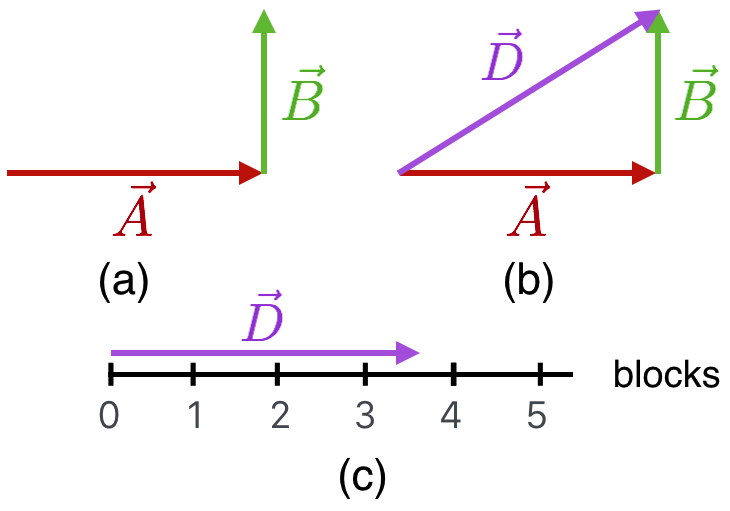
This situation represents a trip through city blocks on the sidewalk: (a) going east \(\vec{A}\) and then north, \(\vec{B}\). Equivalently, (b) represents a trip from the same starting point to the same ending point by cutting across a park, \(\vec{D}\). That third vector is gotten by doing the same tail-to-head manipulation as we did in one dimension. Of course, you’d create that third vector by just walking straight across the park. \(\vec{D}\) is equivalent to the combination of \(\vec{A}\) and \(\vec{B}\), which is to say
Obviously, it’s useful to figure out whether the diagonal path is shorter than the sidewalk paths (thats’ clear by looking) and just how much shorter it is. For that, we need the scale. Let’s use the standard notation that the length (or “magnitude”) of a vector is \(\lvert\vec{V}\rvert\). So here \(\lvert\vec{A}\rvert = 3\) blocks and \(\lvert\vec{B}\rvert = 2\) blocks.
Pens out!
Question! In the figure, how much shorter is cutting across the park as compared to traveling on the sidewalk?
Glad you asked. Obviously the sidewalk journey is \(3 + 2 = 5\) blocks. What’s the length of \(\vec{D}\)? We can do this two ways. One way is to look at the triangle in (b) and remember Pythagoras’ Theorem.
Or we can use the scale, as in (c)…construct \(\vec{D}\) with the head-tail rule and then just transplant it to the scale and see that its length is indeed a little more than 3 and a half. Or, somehow move the scale like a ruler and measure the length of \(\vec{D}\).
Either way, it’s shorter to cut across the park by almost a block and a half. But you sort of knew that.
4.6.3.3. Vector addition in two dimensions, the parallelogram way#
Here’s another situation.
Pens out!
The figure is sort of the same, but means something different. First, the scale says pounds, so it’s two forces \(\vec{A}\) and \(\vec{B}\) but now they’re oriented differently as shown in (a). It seems that Muriel and Earl were unable to get their acts together and so they’re pulling on the dog’s collar at right angles to one another.
So their total pull here is going to be less than 5 pounds and will be some total amount that’s oriented between the two. The (b) figure shows another way to add vectors as a manipulation. Instead of tail to head, (b) shows a placeholder parallelogram drawn in dashed outline and the sum of the two vectors is the diagonal. Of course it’s the same vector you’d get if you’d transported \(\vec{B}\) horizontally to the head of \(\vec{A}\) and added them as before. So this is actually an alternative way to construct vectors sums: the head-to-tail way or the parallelogram way.
4.6.3.4. Decompose a vector#
An inverse of the process of adding two vectors is called resolving or decomposing a vector into its components. This figure shows the steps and is literally the parallelogram addition-method done backwards!
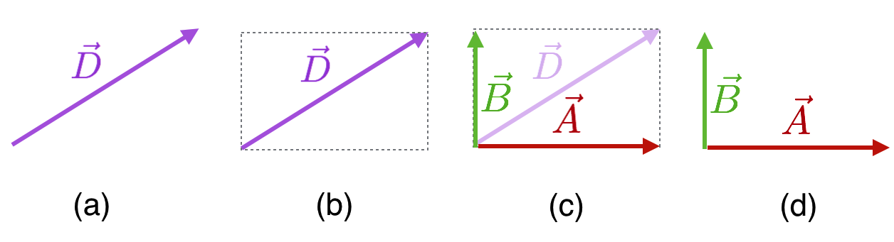
The successive steps involved in 'resolving' a vector into its perpendicular components.
vertical directions (it could be any two directions and they need not be perpendicular). The way to construct this is to add a placeholder parallelogram — usually a rectangle — with the original vector across a diagonal. Then the sides become the two decompositions: the vector components. In both of these cases we’re doing:
Here going from left to right (decomposition of \(\vec{D}\)) and just before, going from right to left (addition of \(\vec{A} \text{ and } \vec{B}\)).
Pens out!
Subtraction of vectors is easy, but requires some thought. In order to construct
We absorb the subtraction sign into the direction designation of \(\vec{D}\) and make a new vector, \(\vec{E} = -\vec{D}.\)…and then add them. This shows the whole sequence of \(\vec{A}-\vec{B} = \vec{A} + \vec{E} = \vec{D}\):
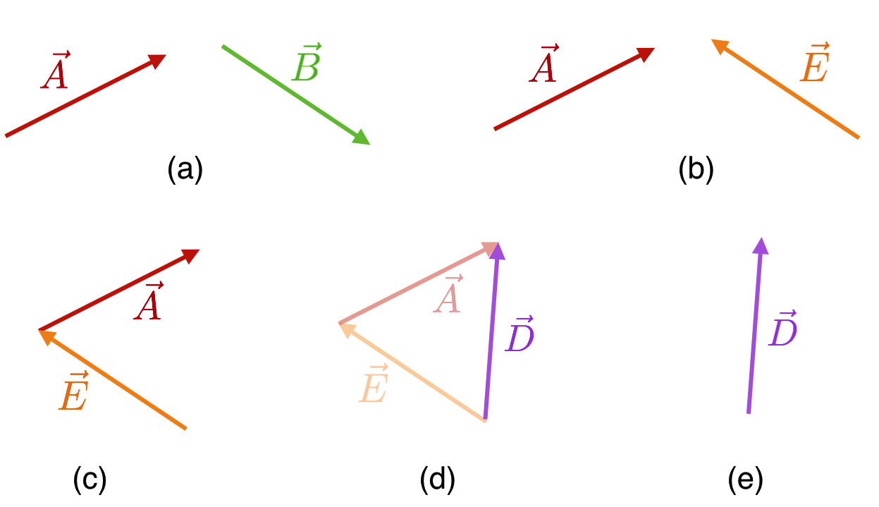
The sequence involved in calculating $\\vec{A} - \\vec{B} = \\vec{D}$
That is everything we’ll need for any vectors that come along in QS&BB!
4.6.4. Approximating Functions#
Pens out!
One skill we’ll need a couple of times is to be able to look at a function and estimate its form for extreme conditions. Here’s what I mean. Look at this perfectly fine function:
We’ll ask this question of a function often:
What is \(y\) if \(x>>b\)
or what is \(y\) if \(x<<b\)?
Here’s the thought process you’d go through to answer these questions. For the first one, if \(x\) is very much larger than \(b\) then that’s nearly asking the question, “What is \(y\) if \(b = 0\)?” which is the extreme of noting that if \(b\) is really tiny compared to \(x\) then it’s almost as if \(b\) isn’t there are all. We’d get:
The other extreme would lead you to say to yourself, “If \(b\) is huge compared to any \(x\), then it’s almost as if \(x\) isn’t there at all.” So:
This kind of analysis can lead to useful insight to the physics of a particular model. But we almost always want to look at a graph, like here, for the special case in which \(a\) and \(b\) are both 1:
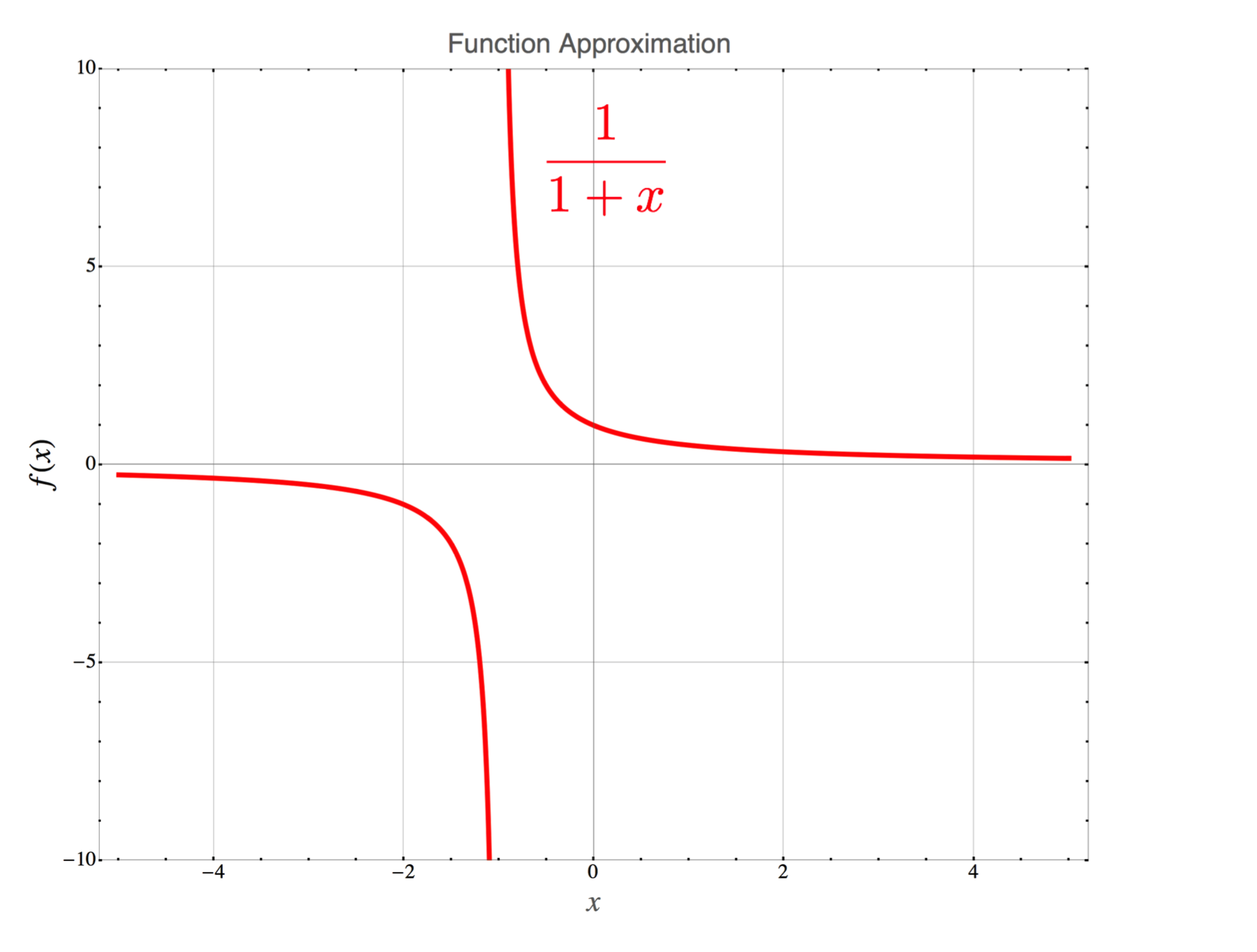
The function $f(x) = \frac{1}{1+x} \nonumber$ which shows exotic behavior when $x=-1$.
For a moment, let’s concentrate on this function for only positive values of \(x\). Then the function looks like this:
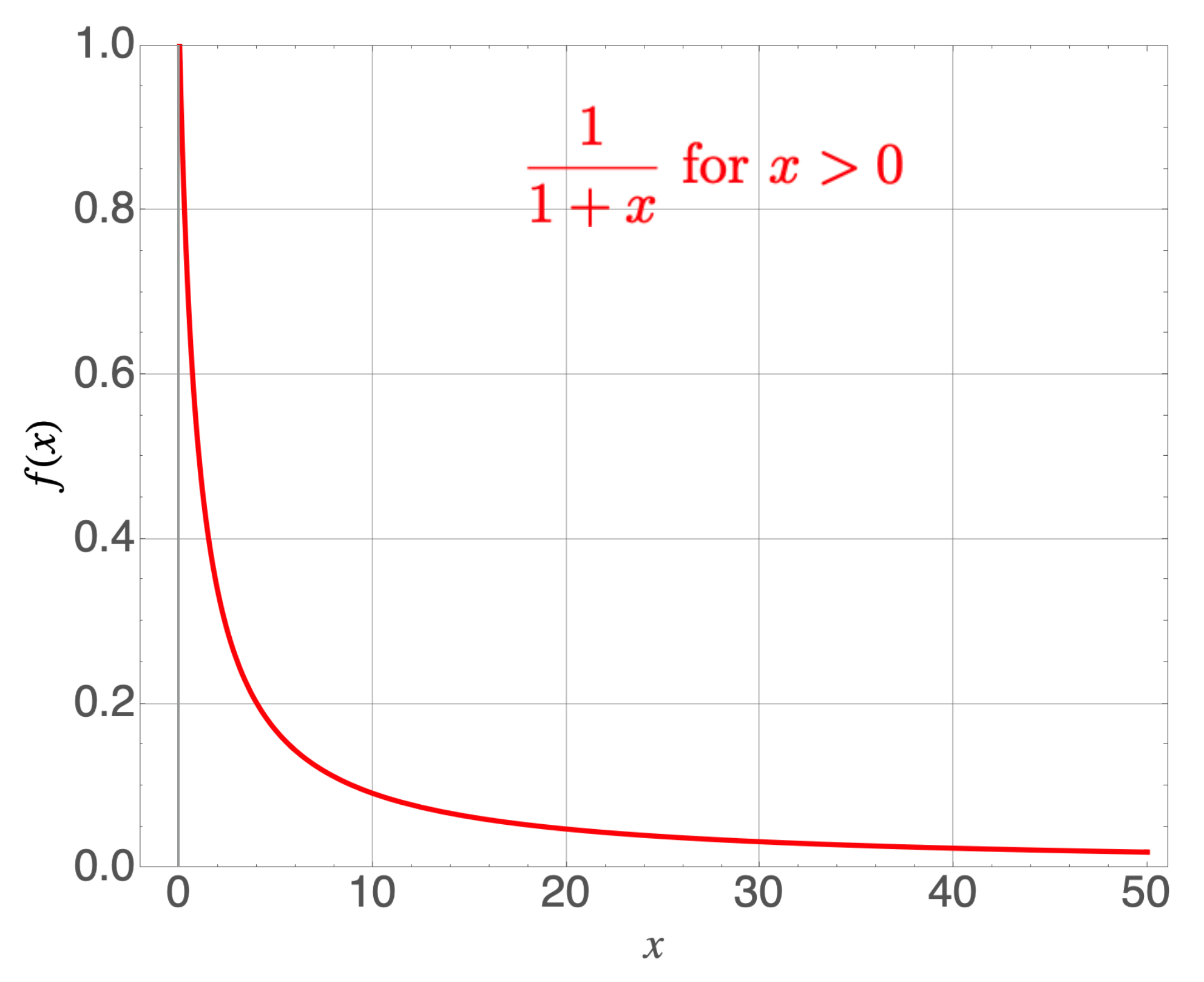
f(x) = \frac{1}{1+x} for values of positive $x$, that is, $x>0$.
Now let’s ask our previous two questions and look for answers in the behavior of the function in this restricted graphical incarnation: when \(x\) gets very very small, the function approaches 1, just as you predicted: \(y(1>>x) \approx \frac{1}{1}.\) Likewise, when \(x\) is enormous, the function gets very small since it now looks like \(y(x>>1) \approx \frac{1}{x}.\)
But there’s a more nuanced way of looking at approximations which is due to Isaac Newton. He found a way to represent a function in pieces, for cases in which the power of such a function could be anything: a positive integer, a negative integer, or even a fraction. The pieces add together to perfectly recreate the original function. The bad news is that to do so perfectly requires an infinite number of them! The good news is that one can get very close to the original function with only a few of the pieces. In contrast to how that sounds, it’s actually very useful for many physics applications as we’ll see.
Here’s his expansion for our function:
That last bit of \(...\) means that the expansion continues in that pattern for an infinite number of terms.
But notice that each term is a separate function in and of itself. That is, \(f(x)\) can be written as the sum and difference of many functions, \(1, x, x^2,...\). Add them all up and you’ll get the original function in all of its glory. Add only the first few terms and you’ll get close to the original function. Let’s do that for the first four terms and compare it to the original, full-fledged function.
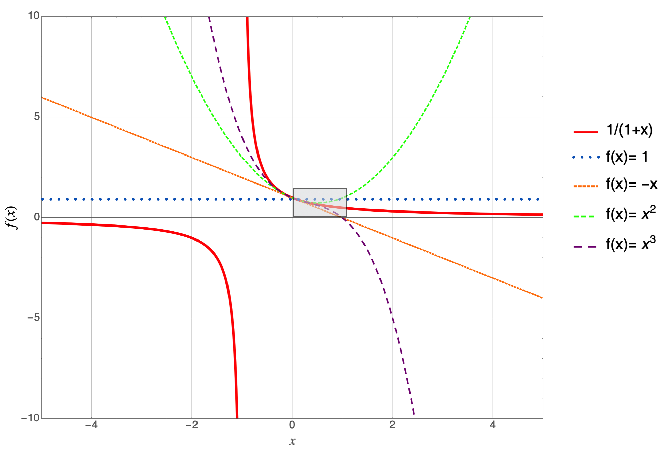
The original function is in solid red and each successive curve adds the next term in the series. So, the blue dotted line is $f(x)=1$, the first term in the series; small dashed orange is adding $-x$, so $f(x)=1-x$; medium dashed green is $f(x)=1-x+x^2$; and finally, long dashed purple is $f(x)=1-x+x^2-x^3$.
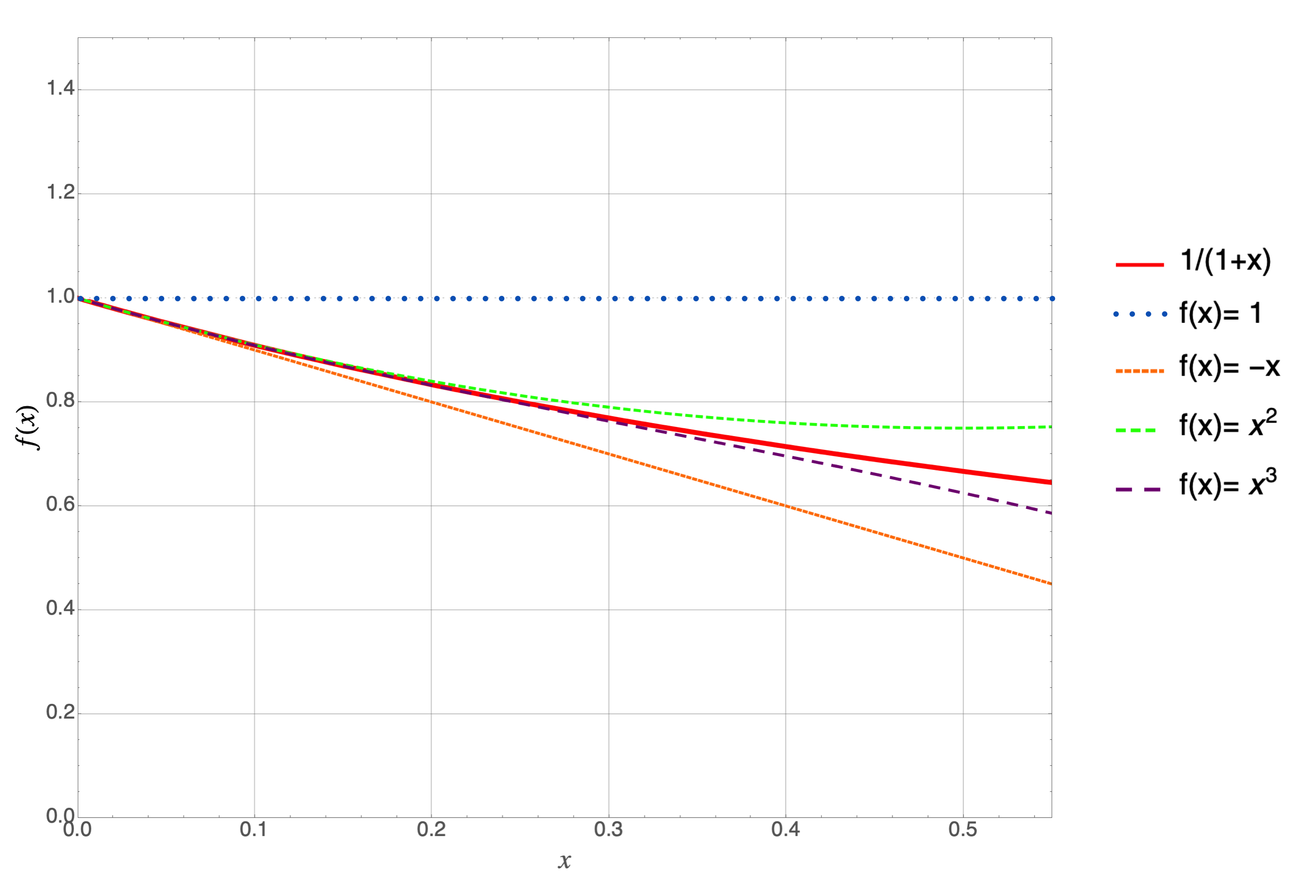
Let’s zoom into the region in the box.
Wait. I’ve had more fun than this…
Glad you asked. Here’s the punchline. You’ll thank me when we get to relativity. Or not.
Suppose that all you cared about was \(x\)’s that are less than about 0.1 and you need to evaluate the curve quickly, or gain some physics insight for that small of an \(x\) region. Then you could get away with approximating
Look at how close the solid red curve is to the short dashed orange curve. Good enough.
Suppose you cared about \(x\)’s that are less than 0.3…then \(1-x\) would not be accurate enough, but the long dashed purple curve would be since it’s indistinguishable from the solid red curve up to that point.
Look how each curve successively makes the approximation better and better as \(x\) increases. So if you can be confident that your \(x\)’s are going to be less than say 0.1, then you can approximate the original function with maybe the first two terms:
since the blue and orange curves when added together are neatly underneath the red curve. The more terms we might add the further out in \(x\) that agreement would continue. Add an infinite number of terms—not advisable—and you’d perfectly reproduce the original function.
Remember this! It will become important later when we’ll encounter some physics functions and approximate them with a few terms of the expansions that we’ll encounter. Here are the functions that we’ll see in the lessons ahead:
Thanks, Isaac.
4.6.5. Formulas From Your Past That Might Only Be Referenced Informally#
Ellipses and hyperbolas will come up, but descriptively. I’ll just want you to have a feel for their shapes and some of the terms that are defined by them. Just file away this location and we’ll come back only a few times.
4.6.5.1. Equation of an ellipse#
An ellipse is a squashed circle (?) that has two axes, the major axis (\(a\)) and the minor axis (\(b\)). The points at which the curve goes through the axes at the major axis points are called the vertices of the ellipse. The equation of an ellipse centered on the origin is
The figure of an ellipse centered on the origin is here:
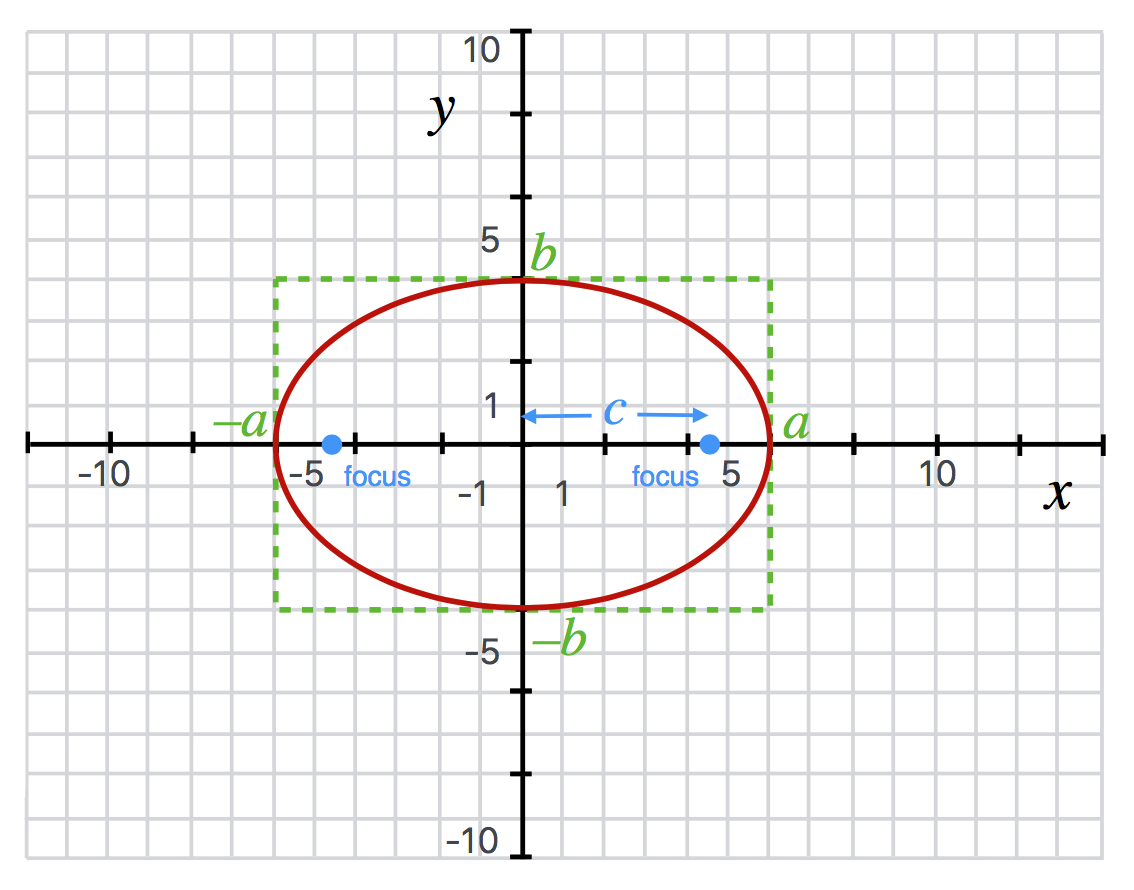
The focus (\(c\) in the diagram) of an ellipse is shown and has the relationship to the curve in that any line connecting one focus to the curve and then to the other focus is always constant. The relationship to the major and minor axes is \(c^2 = a^2-b^2.\) So, if \(a=b\) then the ellipse is actually a circle and the position of the focus is at the center of the circle, here the origin. The degree to which an ellipse is almost-circle-like (more symmetric) and almost-flattened-like is determined by its “eccentricity,” \(e\). It’s defined as \(e = \frac{c}{a}\). So an eccentricity of zero is a circle and the larger the eccentricity, the more the focus point is close to the vertex…and the flatter it is.
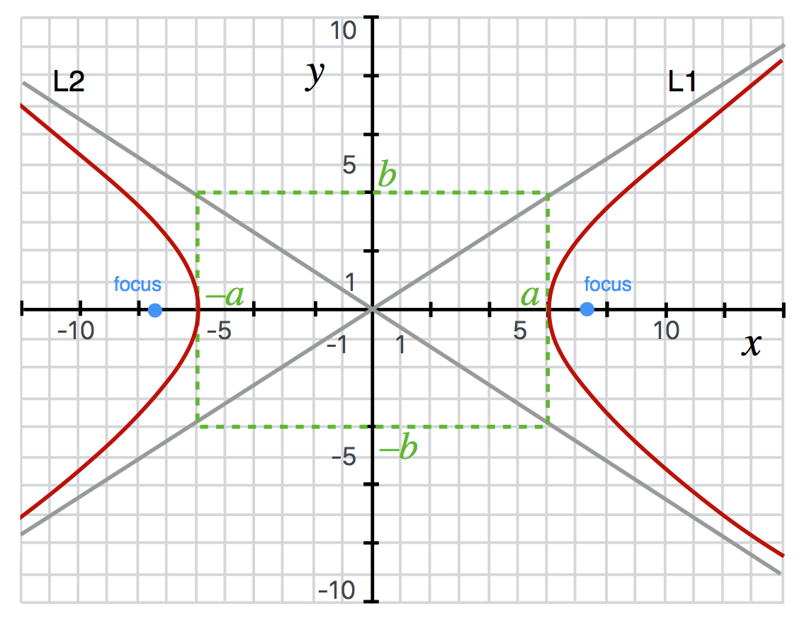
4.6.5.2. Equation of a hyperbola#
I’ll want to refer to a hyperbola once in QS&BB and it will have a particular shape. This particular form of hyperbola is open to the right and left and crosses the \(x\) axis at \(\pm a\)—the “semi-major axis”—and has a semi-minor axis of \(b\) (see the figure). The equation is
The points \((x_0, y_0)\) are where the center of the hyperbola is and in the figure, that’s the origin.
There are a variety of definitions which you can see on the diagram.