5.6. Now For Something Completely Different: Feynman Diagrams#
Richard Feynman was an unusual man. We’ll rely on him periodically as he explains some tough concepts in often bumper-sticker-sized insights. One of the things he did was create a language for dealing with the bizarre concepts of relativistic quantum field theory (a mouthful, but you’ll form those words yourself later) and how we use it to describe the interactions of elementary particles. His language is a sophisticated brand of mathematics, but it comes with a highly visual diagramatic tool that we can use all by itself. It’s already inherent in the graphs we just drew for distance as a function of time for constant speeds. We call that space, Spacetime and Feynman Diagrams are Spacetime Diagrams. Let’s think differently from how you may have before.
5.6.1. Space Diagrams and Spacetime Diagrams#
Ultimately we’ll want to appreciate the collisions of elementary particles and the best image I can think of is a pool table with smooth balls moving around on its surface. Let’s do that. I’ll repeatedly refer to two kinds of geometrical spaces:
Space Diagram. A Space Diagram will be a drawing that a moving object might take in space, for us, \(x\) and \(y\). Sounds simple. If you were to draw the path you took on a road trip you would mark a line on a map with a pencil, following the roads, right? But implicit in this line is that the time that elapsed in your journey is implied, but not explicit. At every mile-marker on the highway you could have marked down the time and it would be more evident. A curve in a Space Diagram is a trajectory in space coordinates where time is kind of in the background.
Spacetime Diagram. A Spacetime Diagram is one in which time is now explicit as one of the coordinates. Since paper is two dimensionally flat for us that means we have to imply one of the formerly evident space dimensions and call out only one of the two (two of the three if we were in three-dimensional space). The result is a Spacetime geometry which only became a thing…with the other guy whom we’ll be constantly referring to, Albert Einstein. Spacetime is a thing…in his Special Theory of Relativity. A trajectory in Spacetime is a curve drawn between points at particular places at a particular times.
A buzzword: “Event.”
An event is a physical happening at a single point in space and at a single time.
If you have a ruler and a clock…you can fully characterize an event. . Touch your screen right here: \(\rightarrow\) x \(\leftarrow\) and look at your watch. The coordinates of the “x” spot and the time that you touched it define that physical act completely.
Another buzzword: “interval.”[1]
We’ll refer to the space and/or time differences between two events as an interval.
Some close-reading here:
Pens out!
Let’s picture a pool table with a single ball engaged in two different interludes. A ball can just sit “still” between two times, minding its own business. A ball can also travel, say, to the right at a constant speed–so it’s at one place at one time and then at a different place at a later time. These are very different circumstances.
This figure shows these two simple interludes [notice the clocks at the top registering the initial time (transparent arrow) and the final time (solid arrow)] as we’d watch them unfold on the table’s surface: at the top (a) the ball is just sitting still and top (b) its moving to the right. In (c) and (d) we see the abstracted Space Diagrams (not pictures of balls, but dots) for each interlude.
The important thing to note is the times. Above each event there’s a clock and two times that have elapsed. In (b), the moving interlude, it’s obvious that the time value at position \((x_0, y_0)\) is \(t_0\) and the time when the ball has traveled to position \((x_1,y_0)\) is \(t_1\). In (a) it’s simpler, but sort of an different way of thinking. The ball is stationary but time…as they say…marches on. I’ve represented that on the same clock face at the top.
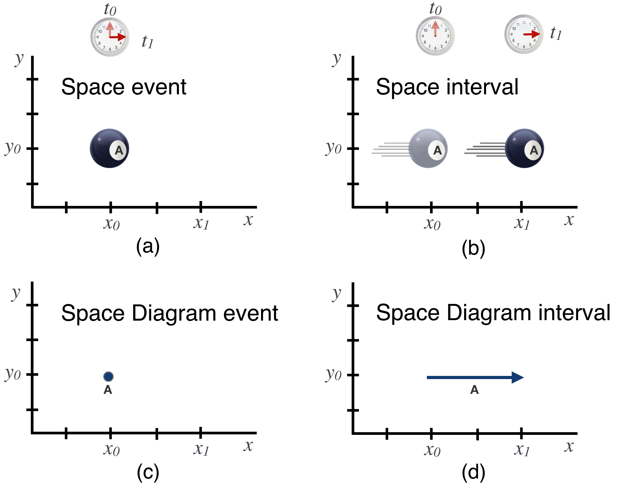
The Space Diagram for event (d) is just exactly that line you’d draw on a map to trace out your journey. The start and the finish points are “events” for us and the space traveled and the time elapsed are “intervals” for us.
This next figure shows a different way of representing these two events.
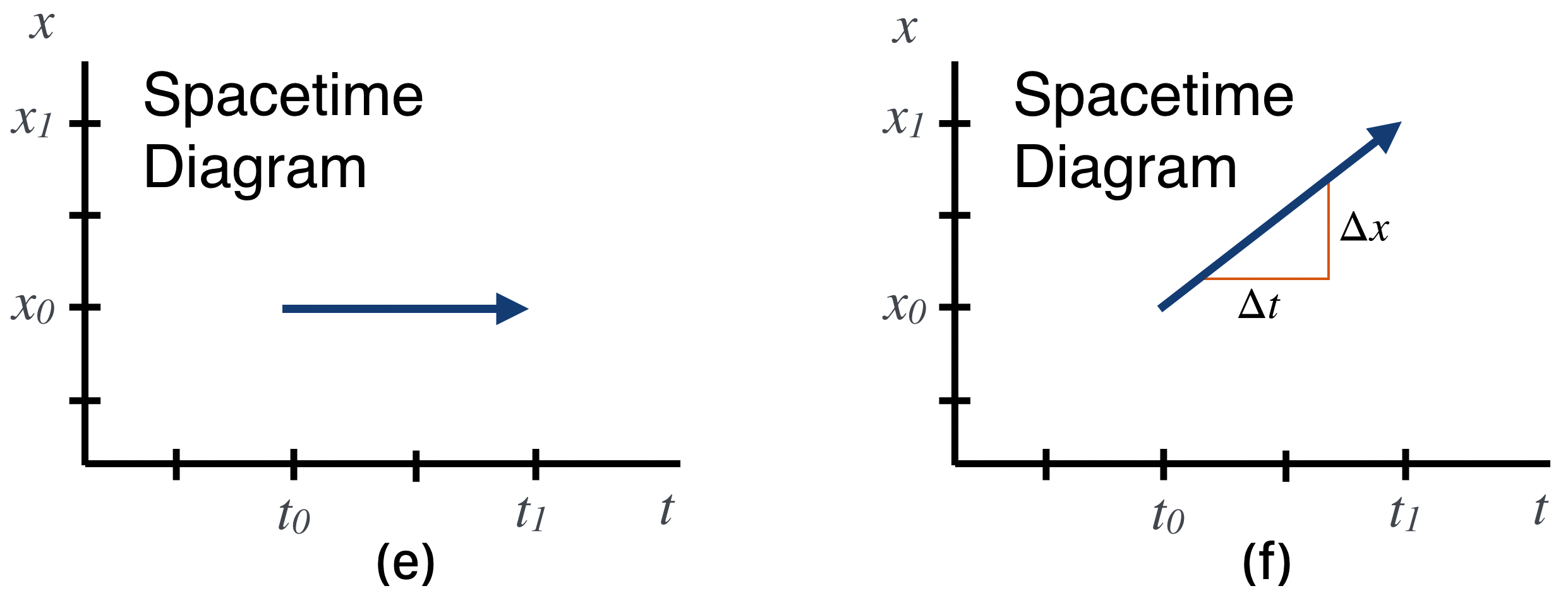
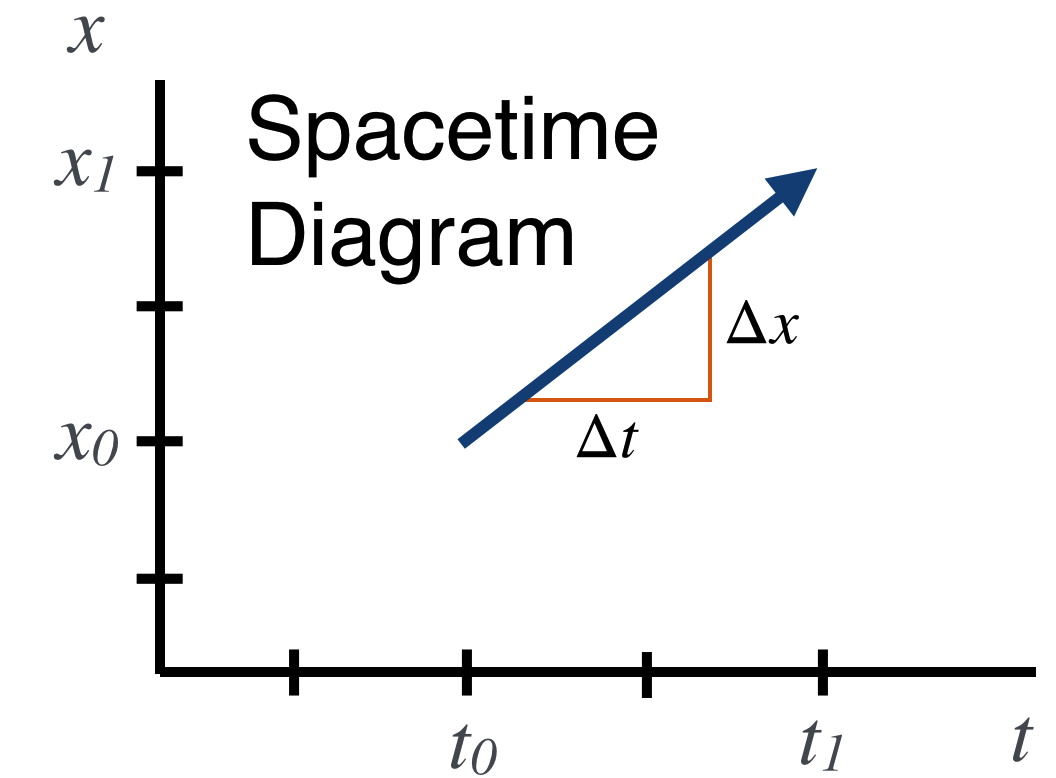
The ball-just-sitting there event in Spacetime is different…the ball in (e) is shown to be stationary in the horizontal space dimension at \(x_0\), but it’s “moving” in the time dimension and the diagram is an arrow through time. For the other event in (f), the Spacetime diagram shows the line that moves forward in time and forward in space and that’s exactly what we’d done earlier. The slope of a properly drawn Spacetime diagram element is the speed of that object. Here I’ve drawn in a slope “calculation”…to guide the eye.
We’re going to love Spacetime diagrams!
We’ll come back to this when we think about colliding things together, when we talk about Relativity, and then again when we talk about actual elementary particle physics collisions in our labs and in the early universe.