7.7. Collision Diagrams: Same Song, Different Verse#
I want us to become familiar with three kinds of diagrams for collisions: space diagrams, spacetime diagrams, and momentum diagrams.
7.7.1. Space Diagram#
Seriously:
Please write the above title and draw the corresponding diagram!
Pens out!
I think that the Space Diagram comes to mind easiest. The next figure is an abstraction of the collision looking down on the table. Notice that as a space diagram, the horizontal and vertical axes are both space lengths.
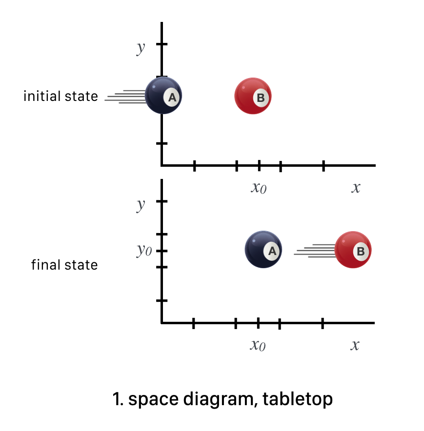
Fig. 7.15 The stop shot at the beginning and the end.#
The next figure shows the trajectories of the initial and final state trajectories. Just like a map…tracing the paths. The dot indicates that a ball is stationary.
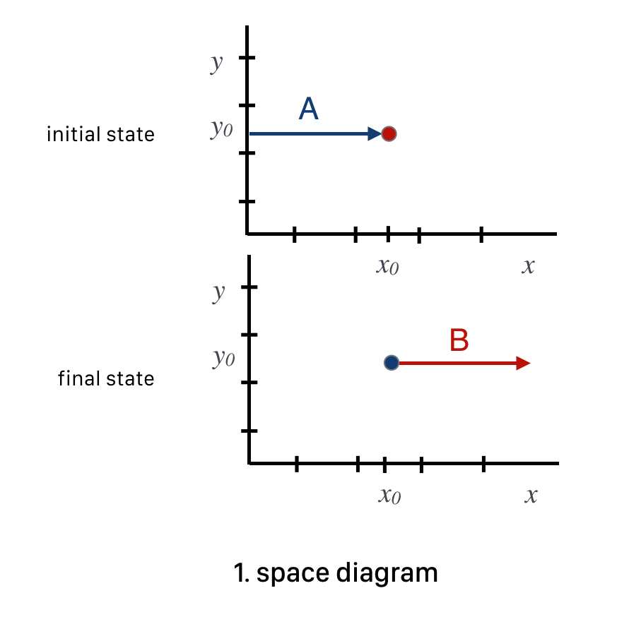
Fig. 7.16 A diagram of the trajectories of the pool balls in the stop shot, of course during some interval of time.#
The coordinates are space distances in both dimensions and time is implied, from the earliest (top) to the latest (bottom) as if snapshots were taken from above the table.
7.7.2. Spacetime Diagram#
Seriously:
Please write the above title and draw the corresponding diagram!
Pens out!
This figure is the Spacetime Diagram for this collision with the vertical axes being one space dimension and the horizontal axes, the time dimension. First, since time is one of the axes, “before” and “after” come for free on one drawing. Second, since this collision happens in one dimension, the vertical \(x\) axis represents all of the action. The \(B\) ball is just sitting still in space at position \(x_0\) but it’s moving in time. Finally, the collision happens at a particular time that’s indicated to be \(t_0\). So \(B\)’s spacetime representation is a horizontal line at \(x_0\) and extending from before \(t_0\) until exactly \(t_C\).
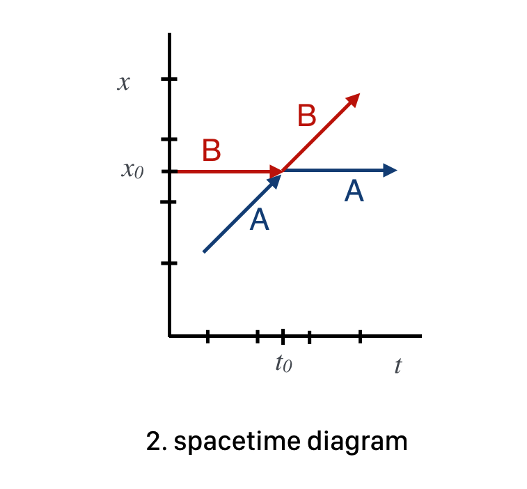
Fig. 7.17 Here we see the spacetime development of the collision. Notice that \( B\) is stationary before it’s hit by \( A\) which is moving (and so slanted in space and time).#
Wait. I’m not sure I see this
Glad you asked. Ah. That’s because you didn’t draw it. Seriously. Drawn the diagram in your notebook and it will become a lot more clear. I’ll wait.
Meanwhile, \(A\) is moving with a positive velocity (the \(x\) distance is increasing in time in a positive sense) and so its speed is represented as a positively sloped line in spacetime. Until \(t_0\). Then \(A\) stops and \(B\) continues with the same velocity that \(A\) enjoyed before it collided with \(B\) and so the slope is the same.
7.7.3. Momentum Diagram#
Seriously:
Please write the above title and draw the corresponding diagram!
It’s also useful to include another diagram…one that represents the collision in a “mathematical space” that’s sort of overlayed on the regular \(x-y\) space but is vectors of momentum, not displacement. Since a momentum vector points in the space \((x,y,z)\) direction of the velocity, we can do this. But now the length of a momentum vector will be the value of the mass times the velocity. This figure is a collection of momentum vectors using our fake units.
Pens out!
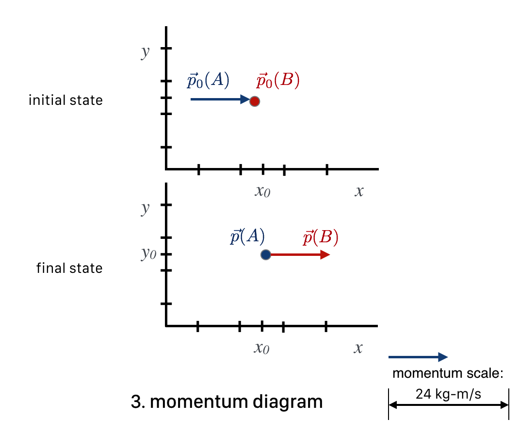
Fig. 7.18 Notice that the scale on the right shows that the blue arrow is half of 24 kg-m/s.#
The key at the bottom shows how long a momentum vector of 24 would be. (In order to emphasize this, I gave our fake momentumunits actual, real units here). Along side of that is an actual momentum vector that’s 12 kg-m/s long.
Look at this. Momentum \(p_0(A)\) is the original “12” momentum of the \(A\) ball and the dot signifies the initial \(B\) momentum as a vector of zero length—no velocity or momentum at all. Likewise, the final state has the situation reversed. Notice that the sum of the momentum vectors in the initial state—the total lengths of the vectors (12 and 0) is equal to the total length of the momentum vectors in the final state. Momentum conservation is expressed as a geometrical relationship among the initial and final state vectors.
Let’s summarize all three diagrams here:
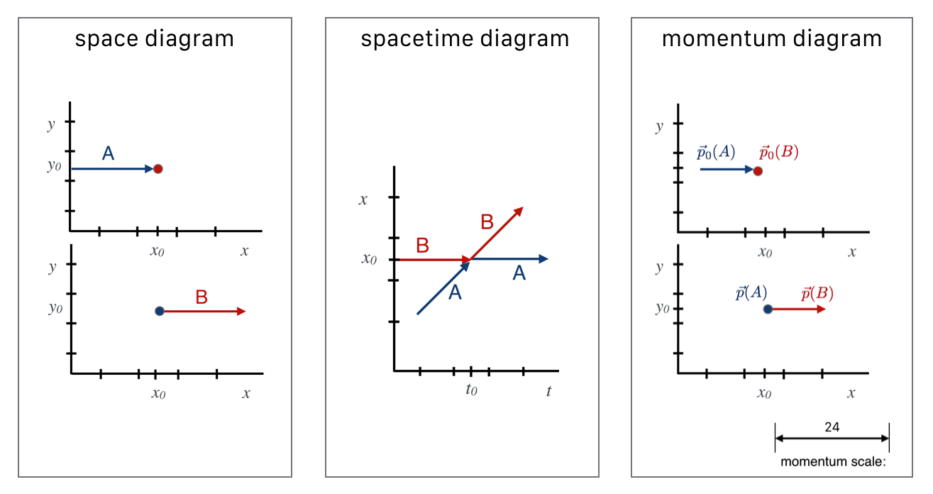
Fig. 7.19 The collection of collision diagrams for the stop-shot collision. All QS&BB collisions can be represented this way.#
Go to 6.6_diagrams_v3_w2m for review and wrap-up of these sections.