4.5. Geometry: Vectors, Curves…Formulas From Your Past?#
4.5.1. Curves#
4.5.1.1. Equation of a circle#
We will deal with some functions that would be very hard to evaluate on your calculator. But Descartes’ gift is that I can show you the graph and evaluation can be done by eye, which is in effect solving the equation. We’ll use some simple geometrical relations which I’ll summarize here.
A circle of radius \(R\) in the \(x-y\) plane centered at a \((a,b)\) is described by the equation:
Of course if the circle is centered at the origin, then it looks more familiar as in this figure:
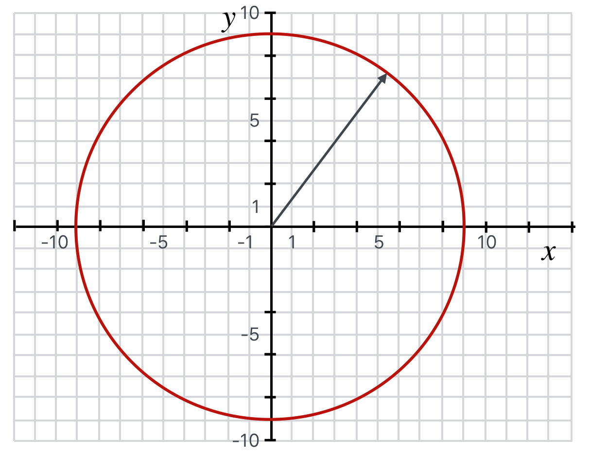
Fig. 4.7 A circle centered at the origin described by the equation, \(x^2 + y^2 = 81\). It has radius of \(9\), area \(A= \\pi 9^2\), and circumference \(C=2 \\pi 9\)#
4.5.1.2. Equation of a parabola#
A parabola in the \(x-y\) plane facing up with vertex at \((a,b)\) where \(C\) is a constant has the equation,
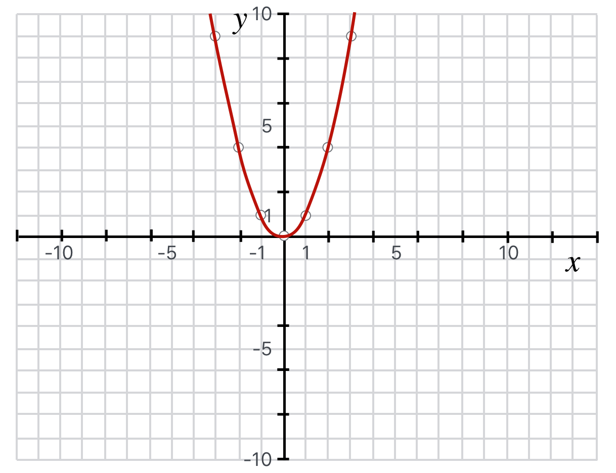
Fig. 4.8 A parabola satisfying the equation, \(y = 1x^2\).#
4.5.1.3. Area of a rectangle#
A rectangle with sides \(a\) and \(b\) has an area, \(A\) of
4.5.1.4. Area of a right triangle#
A right triangle (which means that one of the angles is \(90\) degrees) with base of \(a\) and height of \(b\) has an area, \(A\) of
For a right triangle, the base and height are equal to the two legs. But the formula works for any triangle. Here are some examples,
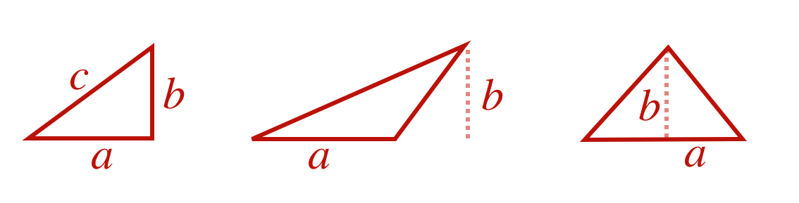
Fig. 4.9 Three triangles, all with the same areas.#
4.5.1.5. Area and circumference of a circle#
Circles will involve \(\pi\) which is an irrational number for which we’ll never need precision better than “March 14th,” \(\pi = 3.14\). And, yes, the story is true that in 1897 Indiana’s General Assembly tried to change the value to \(\pi_{\text{Indiana}}=3.0\) in order to simplfy calculations. Mathematicians and engineers around the state had collective heart palpitations. It disappeared quickly.

Fig. 4.10 You realize that two pizzas is a ‘circumference’? Because…wait for it…it’s ‘2 pie are.’ You’re welcome.#
For a circle of radius \(R\), the area, \(A\) is
and the circumference, \(C\) is
4.5.2. Pythagoras’ Theorem#
For a right triangle (like the left hand triangle above), the hypotenuse, \(c\) is related to the lengths of the two sides \(a\) and \(b\) by the Theorem of Pythagoras:
And, no. He didn’t invent it and it’s been proven many, many different ways.
4.5.3. The quadratic formula#
We might run across a particular polynomial, which you’ve also probably seen before:
It’s an “order 2” polynomial, which means that there are two values of \(x\) that qualify as “solutions”: the values of \(x\) that when substituted make the function be zero. You could plot the function and find what \(x\) values the curve passes through the \(x-\)axis, or you could rely on the time-honored recipe:

Fig. 4.11 You can stop here. The rest is for reference.#