5.4. Calculating a Speed

Some traditional jargon and nomenclature to make your…okay, my life easier. “Change” and “change-of” always means the difference between where you are as compared with where you were. Suppose I start out with $100 and Janet gives me $50. What’s the net change in my net worth? We can represent this simple transaction as

\[\begin{split}\begin{align*} \Delta(\text{my wealth}) &= \text{where I ended up} - \text{where I started} \nonumber \\ &= 150 - 100=50 \text{ ...so I'm up 50 bucks} \nonumber \end{align*}\end{split}\]

which is the definition of our \(\Delta\) : always “the end minus the beginning,” the final value of some quantity minus the initial value of that quantity. Get it?[1]

So let’s apply this to physics and remember … er, a double-remember from Section 3.2 where we defined speed:

\[\text{speed} = \text{distance traveled divided the time that it took}\]

and made it into a simple equation:

\[\text{speed}=\frac{\text{distance traveled}}{\text{time that it took}}.\]

So the numerator is a difference (so we’ll use our difference symbol, \(\Delta\)) of where we ended up in space minus where we started in space:

\[\text{distance traveled in space }=\Delta x = x_{\text{ended up}}-x_{\text{where we started}}.\]

And the denominator is where we ended up in time minus where we started in time:

\[\text{distance traveled in time }= \Delta t = t_{\text{ended up}} - t_{\text{where we started}}.\]

Lots of words, so we’ll use some shorthand.

Using our standard notation in which the “initial state” of any quantity will be decorated with a little “0” subscript, like \(x_0\) here. The “final state” will usually have no subscript and just be \(x\). So

\[\Delta x = x_{\text{ended up}}-x_{\text{where we started}} = x-x_0\]

and

\[\Delta t= t_{\text{ended up}}-t_{\text{when we started}} = t - t_0.\]

So our abstracted model for speed is:

\[v = \frac{\Delta x}{\Delta t}.\]

Boy is Mr. Einstein going to make this interesting.

Sing along Remember the rule. When you see the orange alert “Pens out!” you should open your Notebook and copy what comes next until the orange stripe on the left stops. It’s the path to your brain.

The story of speed

  Pens out!

Let’s work it:

Given what we’ve done this far, using \(\Delta\) notation in the numerator and denominator, we’ve said:

\[ \begin{equation} v = \frac{\Delta x}{\Delta t} = \frac{x - x_0}{t - t_0}. \end{equation}\]

Often, we’ll pretend that we can start our clock at the beginning of some event and so we can usually just let \(t_0=0\) and then the symbol \(t\) just stands for the time interval as well as the ending time. You’ll see.

When you go somewhere, or predict how long it will take to get from one place to another, you would instinctively use an average speed to calculate it. For example, if you travel at a constant 60 mph for 5 hours, how far would you go?

Get out your fingers and your toes for this calculation…it’s \(60 \times 5 = 300\) miles, right? You just did something important. Your brain already knows how to take speed and manipulate it a bit:

\[\begin{split} \begin{align} v &= \frac{\Delta x}{\Delta t} = \frac{x - x_0}{t - t_0} \\ v(t-t_0) & =x-x_0 \\ x-x_0 & =v(t-t_0)=(60)(5)=300 \text{ (miles)}. \end{align} \end{split}\]

More sing along Sometimes when you see a different orange banner that says “Please study Example 1” or some other number, there’s an example for you to go through. You should follow the link and open your Notebook and copy what comes next. This example might be followed by a LON-CAPA question “Please answer Question 1 for points.”

  Please study Example 1:

moving at a constant speed

  Please answer Question 1 for points:

More constant Speed

5.4.1. A Model for Motion

In that example, we’ve just created a model for motion, often an equation and a plot figure prominently in a model. In fact, since:

\[x = x_0 + \langle v \rangle (t - t_0)\]

is the equation for a straight line. Do you remember some time in your past algebraic life saying, “y equals m x plus b” …

\[y=mx + b?\]

Here, “\(y\)” is our distance, \(x\); (briefly, confusingly) \(x\) is our time difference, \(t\); and \(b\) (the slope in the equation) is our average velocity, \(\langle v \rangle\).

So we can see that the straight line from our plots has a slope that’s equivalent to our average speed. Now I don’t know about you, but I can’t drive precisely at 60 mph for 10 minutes, let alone for 5 hours. So here’s a more realistic image of what the distance versus time relation might be.

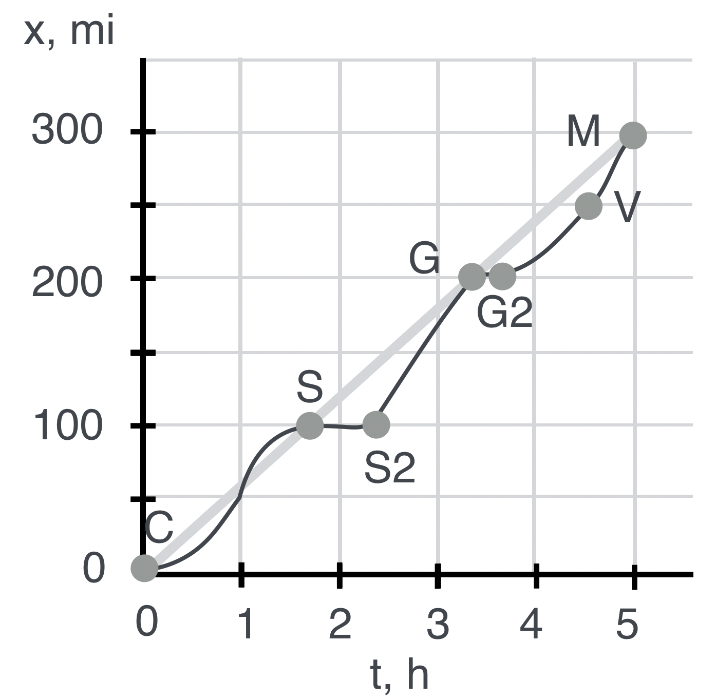
Fig. 5.9 (a) A more realistic (?) trip as the distance varies with time. V is Vanderbilt, Michigan where the speed trap is. (b) What does the speed look like?

Here the dark line is meant to represent a more realistic journey with the light gray line showing the originally ideal, constant velocity trip. Notice that we start slow and speed up and then at Saginaw we stop for dinner: the distance is unchanged for almost an hour until point S2 when we start up again. And boy, do we ever. We fly through Grayling (G) on to Vanderbilt (V) and then more slowly, get to the bridge.

Let’s analyze this while feeling sorry for ourselves about that speeding ticket.

  Please study Example 2:

realistic trip

  Please answer Question 2 for points:

Real trip

Can you see that the average speed is the same for the realistic trajectory and the originally idealistic steady-on-the-gas picture? All the average depends on is the beginning and the end.

Instantaneous speed If you want to know more details, then you’d need shorter time intervals. In each successively smaller interval you’d know the speed more precisely and in the limit where you’re just at a point on some curve of distance – well, that’s the instantaneous speed. That too is an idealistic notion since any measurement of speed would require a finite time interval. Of course your speedometer is calculating an average also, but the time interval is so short that we tend to think of the reading in the cockpit as our speed right now.

  Pens out!

So now we have a functional relationship that acts as a little calculating engine: you give me a time and a speed and your starting point, I’ll reliably tell you your new position when your clock reaches that time. The world can be pretty neat that way. Here it is:

\[x = x_0+\langle v \rangle t\]

Often we’ll be a little casual about the average sign and we’d just say

\[x = x_0+ v t.\]

This is how we’ll use models in QS&BB: sometimes an equation, but most times, a plot of an equation.

---

[1]

So if class starts at 10:20 AM and if I were to fall asleep in mid-sentence at 10:50, it would be embarrassing. When you posted my snoring image to Instagram you’d calculate that \(t_0=10:20\) and \(t=10:50\) and so you’d report that I managed to stay awake for \(\Delta t=t - t_0 = 30\) minutes.