Collisions#
Example 3: A Real Collision 2: \(\mathbf{ a}+\mathbf{B}\to \mathbf{a}+\mathbf{B}\)#
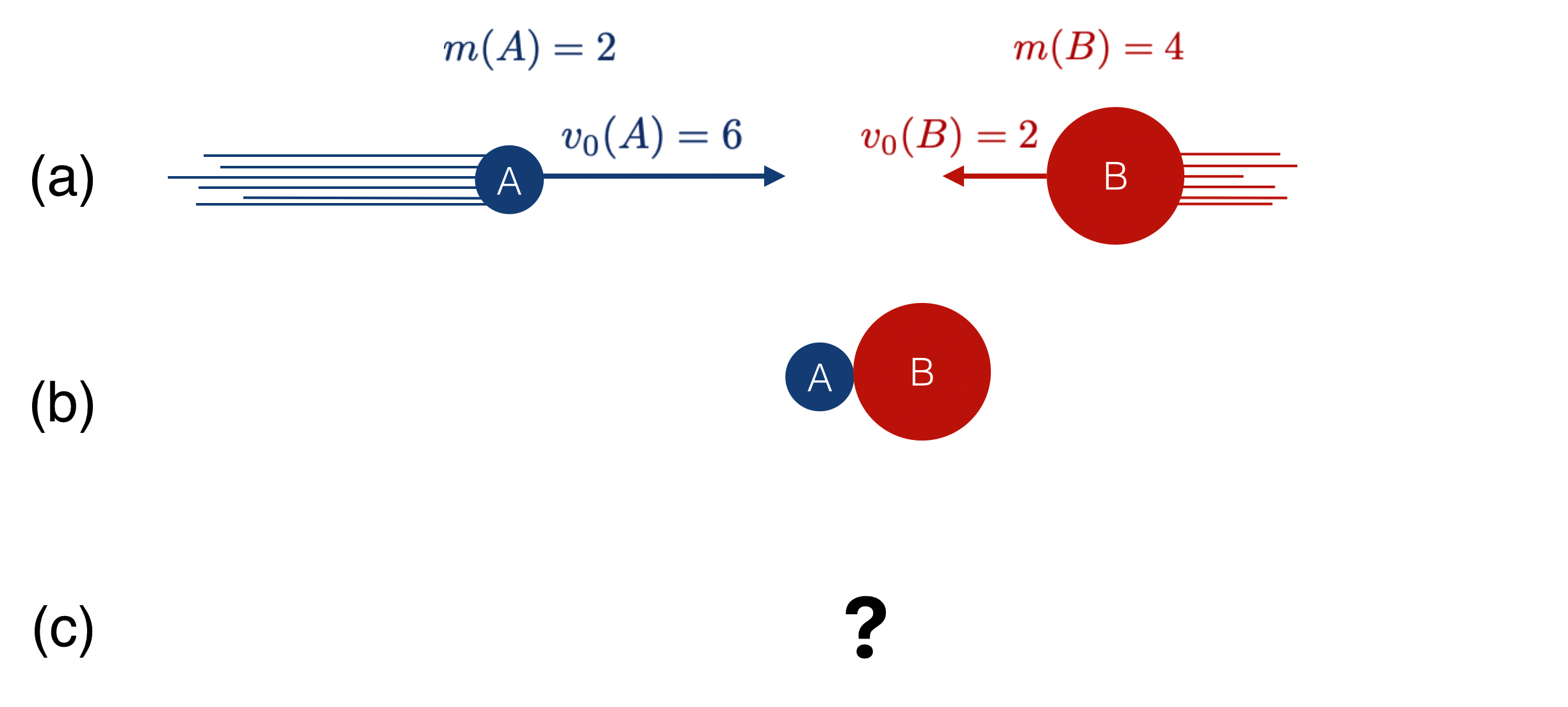
Angus (we’ll call him \(A\), rather than \(a\)) is a slight, but quick football safety trying to tackle Buster (\(B\)), the huge running back. Angus bounces off the lumbering Buster. (It could also be a small car and a large truck, but that’s too scary.)
This is not a tackle (because they’d become a single entity in a tackle). Rather this is a bounce in which Angus and Buster will be separate.
Here are the data for this collision, again with fake units:
\(m(A)= 2\) and \(v_0(A)=6\)
\(m(B)= 4\) and \(v_0(B)=2\) the other way… so if we take \(A\)’s direction to be positive, then \(\vec{v}_0(B)=-2\), or since we’re in one dimension, \(v_0(B)=-2\)
So, \(p_0(A)= 2\times 6 = 12\)
and \(p_0(B)= 4\times (-2) = -8\)
The final piece of data that I’ll tell you that Angus’
final momentum is \(p(A) =-9.3\): so, he bounces back, off of Buster.
The operative football question for the defense, is whether Angus pushed Buster backwards for a loss or does he still carry his momentum forward for a gain.
Questions:
What’s Angus’s final velocity?
What is Buster’s final momentum after colliding with Angus?
Answers:
What is \(A\)’s final velocity?
Our intrepid (courageous!) Angus’s final velocity is easy. We know his mass (\(m(A)=2\) and his momentum \(p(A)=-9.3\), so we can get his velocity one of two ways:
calculate it:
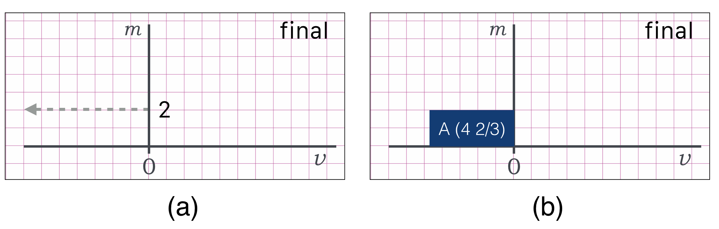
\[\begin{split} \begin{align*} p(A) &=-9.3 = m(A)v(A) \\ v(A) &= \frac{p(A)}{m(A)} \\ v(A) &= \frac{-9.3}{2} = -4.67 \end{align*} \end{split}\]or use an area plot. Set up an \(m\) versus \(v\) set of axes…draw a horizontal line at the known value of \(m=2\) and construct the rectangular area to be the known momentum of \(9.3\):
What’s \(B\)’s momentum after the collision?
We could create areas and solve this but I think that more insight comes quickest if we use the thermometer approach. Here’s our construction:
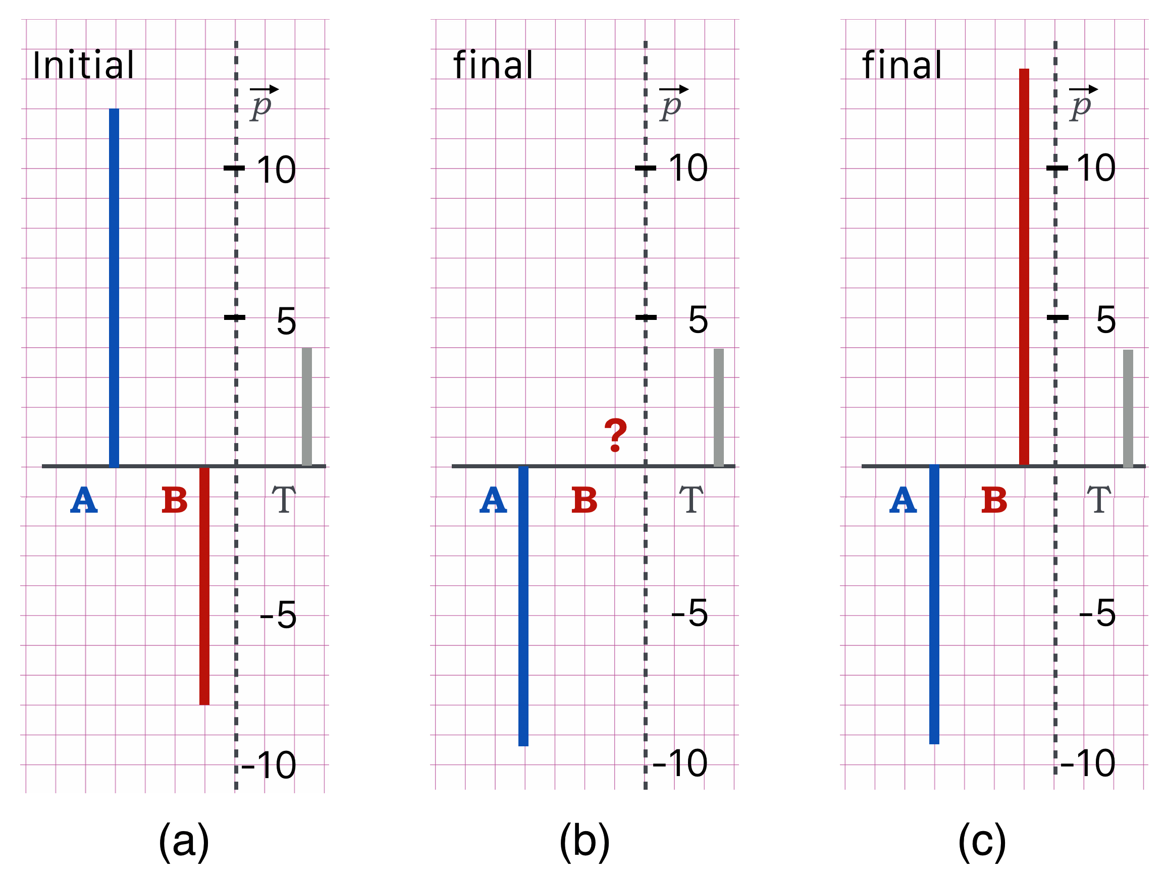
And, here’s my reasoning:
In (a) I’ve plotted the initial momenta for each object. Angus with a positive momentum of 12 and Buster with his negative momentum of \(-8\).
The total momentum of the Angus-Buster system is the sum, which I can represent as the sum of the two thermometer lines, here the difference since one is negative.
I can quickly see that the difference of those momenta leaves \(4\), which is then the absolute total, \(p(T)=4\). So the combination of the final momenta also have to sum to be that same value–momentum conservation.
In (a) then, on the right hand side, I’ve put in the thermometer for that difference: \(p(T)=4\).
That’s our initial situation and the key is creating that \(T\) thermometer as the total…which has to be the same total in the final state, which is in the middle diagram, (b):
I know the final \(A\) momentum, and that’s added in (b) and I brought along \(T\) on the right: because THAT’s the statement of momentum conservation!
So we can construct \(B\)’s momentum which, when combined with that of \(A\) will give us \(T\) again.
That’s shown in (c). Count up the squares for \(B\) and you’ll see that \(P(B)=\text{about }13.3.\)
With pictures I’m solving the momentum conservation equations:
Either approach is fine!